

11.6: 2nd order Rate Laws
- Page ID
- 84363
\( \newcommand{\vecs}[1]{\overset { \scriptstyle \rightharpoonup} {\mathbf{#1}} } \)
\( \newcommand{\vecd}[1]{\overset{-\!-\!\rightharpoonup}{\vphantom{a}\smash {#1}}} \)
\( \newcommand{\id}{\mathrm{id}}\) \( \newcommand{\Span}{\mathrm{span}}\)
( \newcommand{\kernel}{\mathrm{null}\,}\) \( \newcommand{\range}{\mathrm{range}\,}\)
\( \newcommand{\RealPart}{\mathrm{Re}}\) \( \newcommand{\ImaginaryPart}{\mathrm{Im}}\)
\( \newcommand{\Argument}{\mathrm{Arg}}\) \( \newcommand{\norm}[1]{\| #1 \|}\)
\( \newcommand{\inner}[2]{\langle #1, #2 \rangle}\)
\( \newcommand{\Span}{\mathrm{span}}\)
\( \newcommand{\id}{\mathrm{id}}\)
\( \newcommand{\Span}{\mathrm{span}}\)
\( \newcommand{\kernel}{\mathrm{null}\,}\)
\( \newcommand{\range}{\mathrm{range}\,}\)
\( \newcommand{\RealPart}{\mathrm{Re}}\)
\( \newcommand{\ImaginaryPart}{\mathrm{Im}}\)
\( \newcommand{\Argument}{\mathrm{Arg}}\)
\( \newcommand{\norm}[1]{\| #1 \|}\)
\( \newcommand{\inner}[2]{\langle #1, #2 \rangle}\)
\( \newcommand{\Span}{\mathrm{span}}\) \( \newcommand{\AA}{\unicode[.8,0]{x212B}}\)
\( \newcommand{\vectorA}[1]{\vec{#1}} % arrow\)
\( \newcommand{\vectorAt}[1]{\vec{\text{#1}}} % arrow\)
\( \newcommand{\vectorB}[1]{\overset { \scriptstyle \rightharpoonup} {\mathbf{#1}} } \)
\( \newcommand{\vectorC}[1]{\textbf{#1}} \)
\( \newcommand{\vectorD}[1]{\overrightarrow{#1}} \)
\( \newcommand{\vectorDt}[1]{\overrightarrow{\text{#1}}} \)
\( \newcommand{\vectE}[1]{\overset{-\!-\!\rightharpoonup}{\vphantom{a}\smash{\mathbf {#1}}}} \)
\( \newcommand{\vecs}[1]{\overset { \scriptstyle \rightharpoonup} {\mathbf{#1}} } \)
\( \newcommand{\vecd}[1]{\overset{-\!-\!\rightharpoonup}{\vphantom{a}\smash {#1}}} \)
\(\newcommand{\avec}{\mathbf a}\) \(\newcommand{\bvec}{\mathbf b}\) \(\newcommand{\cvec}{\mathbf c}\) \(\newcommand{\dvec}{\mathbf d}\) \(\newcommand{\dtil}{\widetilde{\mathbf d}}\) \(\newcommand{\evec}{\mathbf e}\) \(\newcommand{\fvec}{\mathbf f}\) \(\newcommand{\nvec}{\mathbf n}\) \(\newcommand{\pvec}{\mathbf p}\) \(\newcommand{\qvec}{\mathbf q}\) \(\newcommand{\svec}{\mathbf s}\) \(\newcommand{\tvec}{\mathbf t}\) \(\newcommand{\uvec}{\mathbf u}\) \(\newcommand{\vvec}{\mathbf v}\) \(\newcommand{\wvec}{\mathbf w}\) \(\newcommand{\xvec}{\mathbf x}\) \(\newcommand{\yvec}{\mathbf y}\) \(\newcommand{\zvec}{\mathbf z}\) \(\newcommand{\rvec}{\mathbf r}\) \(\newcommand{\mvec}{\mathbf m}\) \(\newcommand{\zerovec}{\mathbf 0}\) \(\newcommand{\onevec}{\mathbf 1}\) \(\newcommand{\real}{\mathbb R}\) \(\newcommand{\twovec}[2]{\left[\begin{array}{r}#1 \\ #2 \end{array}\right]}\) \(\newcommand{\ctwovec}[2]{\left[\begin{array}{c}#1 \\ #2 \end{array}\right]}\) \(\newcommand{\threevec}[3]{\left[\begin{array}{r}#1 \\ #2 \\ #3 \end{array}\right]}\) \(\newcommand{\cthreevec}[3]{\left[\begin{array}{c}#1 \\ #2 \\ #3 \end{array}\right]}\) \(\newcommand{\fourvec}[4]{\left[\begin{array}{r}#1 \\ #2 \\ #3 \\ #4 \end{array}\right]}\) \(\newcommand{\cfourvec}[4]{\left[\begin{array}{c}#1 \\ #2 \\ #3 \\ #4 \end{array}\right]}\) \(\newcommand{\fivevec}[5]{\left[\begin{array}{r}#1 \\ #2 \\ #3 \\ #4 \\ #5 \\ \end{array}\right]}\) \(\newcommand{\cfivevec}[5]{\left[\begin{array}{c}#1 \\ #2 \\ #3 \\ #4 \\ #5 \\ \end{array}\right]}\) \(\newcommand{\mattwo}[4]{\left[\begin{array}{rr}#1 \amp #2 \\ #3 \amp #4 \\ \end{array}\right]}\) \(\newcommand{\laspan}[1]{\text{Span}\{#1\}}\) \(\newcommand{\bcal}{\cal B}\) \(\newcommand{\ccal}{\cal C}\) \(\newcommand{\scal}{\cal S}\) \(\newcommand{\wcal}{\cal W}\) \(\newcommand{\ecal}{\cal E}\) \(\newcommand{\coords}[2]{\left\{#1\right\}_{#2}}\) \(\newcommand{\gray}[1]{\color{gray}{#1}}\) \(\newcommand{\lgray}[1]{\color{lightgray}{#1}}\) \(\newcommand{\rank}{\operatorname{rank}}\) \(\newcommand{\row}{\text{Row}}\) \(\newcommand{\col}{\text{Col}}\) \(\renewcommand{\row}{\text{Row}}\) \(\newcommand{\nul}{\text{Nul}}\) \(\newcommand{\var}{\text{Var}}\) \(\newcommand{\corr}{\text{corr}}\) \(\newcommand{\len}[1]{\left|#1\right|}\) \(\newcommand{\bbar}{\overline{\bvec}}\) \(\newcommand{\bhat}{\widehat{\bvec}}\) \(\newcommand{\bperp}{\bvec^\perp}\) \(\newcommand{\xhat}{\widehat{\xvec}}\) \(\newcommand{\vhat}{\widehat{\vvec}}\) \(\newcommand{\uhat}{\widehat{\uvec}}\) \(\newcommand{\what}{\widehat{\wvec}}\) \(\newcommand{\Sighat}{\widehat{\Sigma}}\) \(\newcommand{\lt}{<}\) \(\newcommand{\gt}{>}\) \(\newcommand{\amp}{&}\) \(\definecolor{fillinmathshade}{gray}{0.9}\)If the reaction follows a second order rate law, the some methodology can be employed. The rate can be written as
\[ -\dfrac{d[A]}{dt} = k [A]^2 \label{eq1A} \]
The separation of concentration and time terms (this time keeping the negative sign on the left for convenience) yields
\[ -\dfrac{d[A]}{[A]^2} = k \,dt \nonumber \]
The integration then becomes
\[ - \int_{[A]_o}^{[A]} \dfrac{d[A]}{[A]^2} = \int_{t=0}^{t}k \,dt \label{eq1} \]
And noting that
\[ - \dfrac{dx}{x^2} = d \left(\dfrac{1}{x} \right) \nonumber \]
the result of integration Equation \ref{eq1} is
\[ \dfrac{1}{[A]} -\dfrac{1}{[A]_o} = kt \nonumber \]
or
\[ \dfrac{1}{[A]} = \dfrac{1}{[A]_o} + kt \nonumber \]
And so a plot of \(1/[A]\) as a function of time should produce a linear plot, the slope of which is \(k\), and the intercept of which is \(1/[A]_0\).
Other 2nd order rate laws are a little bit trickier to integrate, as the integration depends on the actual stoichiometry of the reaction being investigated. For example, for a reaction of the type
\[A + B \rightarrow P \nonumber \]
That has rate laws given by
\[ -\dfrac{d[A]}{dt} = k [A][B] \nonumber \]
and
\[ -\dfrac{d[B]}{dt} = k [A][B] \nonumber \]
the integration will depend on the decrease of [A] and [B] (which will be related by the stoichiometry) which can be expressed in terms the concentration of the product [P].
\[[A] = [A]_o – [P] \label{eqr1} \]
and
\[[B] = [B]_o – [P]\label{eqr2} \]
The concentration dependence on \(A\) and \(B\) can then be eliminated if the rate law is expressed in terms of the production of the product.
\[ \dfrac{d[P]}{dt} = k [A][B] \label{rate2} \]
Substituting the relationships for \([A]\) and \([B]\) (Equations \ref{eqr1} and \ref{eqr2}) into the rate law expression (Equation \ref{rate2}) yields
\[ \dfrac{d[P]}{dt} = k ( [A]_o – [P]) ([B] = [B]_o – [P]) \label{rate3} \]
Separation of concentration and time variables results in
\[\dfrac{d[P]}{( [A]_o – [P]) ([B] = [B]_o – [P])} = k\,dt \nonumber \]
Noting that at time \(t = 0\), \([P] = 0\), the integrated form of the rate law can be generated by solving the integral
\[\int_{[A]_o}^{[A]} \dfrac{d[P]}{( [A]_o – [P]) ([B]_o – [P])} = \int_{t=0}^{t} k\,dt \nonumber \]
Consulting a table of integrals reveals that for \(a \neq b\)[1],
\[ \int \dfrac{dx}{(a-x)(b-x)} = \dfrac{1}{b-a} \ln \left(\dfrac{b-x}{a-x} \right) \nonumber \]
Applying the definite integral (as long as \([A]_0 \neq [B]_0\)) results in
\[ \left. \dfrac{1}{[B]_0-[A]_0} \ln \left( \dfrac{[B]_0-[P]}{[A]_0-[P]} \right) \right |_0^{[A]} = \left. k\, t \right|_0^t \nonumber \]
\[ \dfrac{1}{[B]_0-[A]_0} \ln \left( \dfrac{[B]_0-[P]}{[A]_0-[P]} \right) -\dfrac{1}{[B]_0-[A]_0} \ln \left( \dfrac{[B]_0}{[A]_0} \right) =k\, t \label{finalint} \]
Substituting Equations \ref{eqr1} and \ref{eqr2} into Equation \ref{finalint} and simplifying (combining the natural logarithm terms) yields
\[\dfrac{1}{[B]_0-[A]_0} \ln \left( \dfrac{[B][A]_o}{[A][B]_o} \right) = kt \nonumber \]
For this rate law, a plot of \(\ln([B]/[A])\) as a function of time will produce a straight line, the slope of which is
\[ m = ([B]_0 – [A]_0)k. \nonumber \]
In the limit at \([A]_0 = [B]_0\), then \([A] = [B]\) at all times, due to the stoichiometry of the reaction. As such, the rate law becomes
\[ \text{rate} = k [A]^2 \nonumber \]
and integrate direct like in Equation \ref{eq1A} and the integrated rate law is (as before)
\[ \dfrac{1}{[A]} = \dfrac{1}{[A]_o} + kt \nonumber \]
Consider the following kinetic data. Use a graph to demonstrate that the data are consistent with second order kinetics. Also, if the data are second order, determine the value of the rate constant for the reaction.
| time (s) | 0 | 10 | 30 | 60 | 100 | 150 | 200 |
|---|---|---|---|---|---|---|---|
| [A] (M) | 0.238 | 0.161 | 0.098 | 0.062 | 0.041 | 0.029 | 0.023 |
Solution
The plot looks as follows:
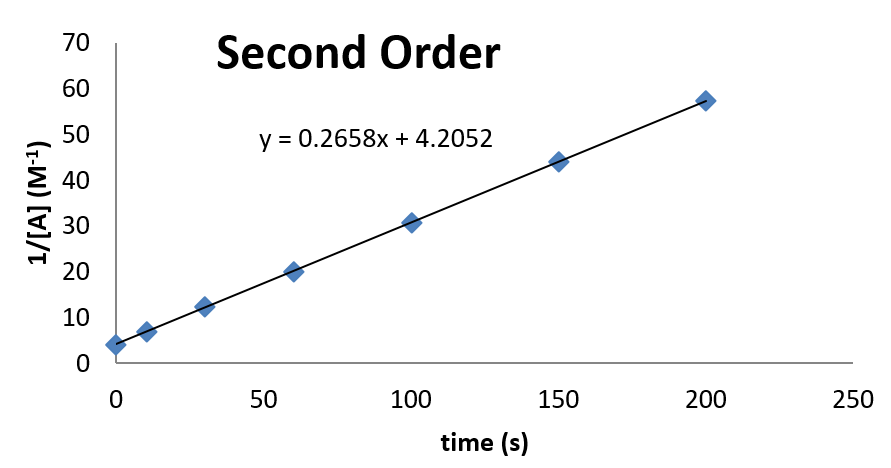
From this plot, it can be seen that the rate constant is 0.2658 M-1 s-1. The concentration at time \(t = 0\) can also be inferred from the intercept.
[1] This integral form can be generated by using the method of partial fractions. See (House, 2007) for a full derivation.