5.2: Heat Engines and the Carnot Cycle
- Page ID
- 84317
\( \newcommand{\vecs}[1]{\overset { \scriptstyle \rightharpoonup} {\mathbf{#1}} } \)
\( \newcommand{\vecd}[1]{\overset{-\!-\!\rightharpoonup}{\vphantom{a}\smash {#1}}} \)
\( \newcommand{\id}{\mathrm{id}}\) \( \newcommand{\Span}{\mathrm{span}}\)
( \newcommand{\kernel}{\mathrm{null}\,}\) \( \newcommand{\range}{\mathrm{range}\,}\)
\( \newcommand{\RealPart}{\mathrm{Re}}\) \( \newcommand{\ImaginaryPart}{\mathrm{Im}}\)
\( \newcommand{\Argument}{\mathrm{Arg}}\) \( \newcommand{\norm}[1]{\| #1 \|}\)
\( \newcommand{\inner}[2]{\langle #1, #2 \rangle}\)
\( \newcommand{\Span}{\mathrm{span}}\)
\( \newcommand{\id}{\mathrm{id}}\)
\( \newcommand{\Span}{\mathrm{span}}\)
\( \newcommand{\kernel}{\mathrm{null}\,}\)
\( \newcommand{\range}{\mathrm{range}\,}\)
\( \newcommand{\RealPart}{\mathrm{Re}}\)
\( \newcommand{\ImaginaryPart}{\mathrm{Im}}\)
\( \newcommand{\Argument}{\mathrm{Arg}}\)
\( \newcommand{\norm}[1]{\| #1 \|}\)
\( \newcommand{\inner}[2]{\langle #1, #2 \rangle}\)
\( \newcommand{\Span}{\mathrm{span}}\) \( \newcommand{\AA}{\unicode[.8,0]{x212B}}\)
\( \newcommand{\vectorA}[1]{\vec{#1}} % arrow\)
\( \newcommand{\vectorAt}[1]{\vec{\text{#1}}} % arrow\)
\( \newcommand{\vectorB}[1]{\overset { \scriptstyle \rightharpoonup} {\mathbf{#1}} } \)
\( \newcommand{\vectorC}[1]{\textbf{#1}} \)
\( \newcommand{\vectorD}[1]{\overrightarrow{#1}} \)
\( \newcommand{\vectorDt}[1]{\overrightarrow{\text{#1}}} \)
\( \newcommand{\vectE}[1]{\overset{-\!-\!\rightharpoonup}{\vphantom{a}\smash{\mathbf {#1}}}} \)
\( \newcommand{\vecs}[1]{\overset { \scriptstyle \rightharpoonup} {\mathbf{#1}} } \)
\( \newcommand{\vecd}[1]{\overset{-\!-\!\rightharpoonup}{\vphantom{a}\smash {#1}}} \)
\(\newcommand{\avec}{\mathbf a}\) \(\newcommand{\bvec}{\mathbf b}\) \(\newcommand{\cvec}{\mathbf c}\) \(\newcommand{\dvec}{\mathbf d}\) \(\newcommand{\dtil}{\widetilde{\mathbf d}}\) \(\newcommand{\evec}{\mathbf e}\) \(\newcommand{\fvec}{\mathbf f}\) \(\newcommand{\nvec}{\mathbf n}\) \(\newcommand{\pvec}{\mathbf p}\) \(\newcommand{\qvec}{\mathbf q}\) \(\newcommand{\svec}{\mathbf s}\) \(\newcommand{\tvec}{\mathbf t}\) \(\newcommand{\uvec}{\mathbf u}\) \(\newcommand{\vvec}{\mathbf v}\) \(\newcommand{\wvec}{\mathbf w}\) \(\newcommand{\xvec}{\mathbf x}\) \(\newcommand{\yvec}{\mathbf y}\) \(\newcommand{\zvec}{\mathbf z}\) \(\newcommand{\rvec}{\mathbf r}\) \(\newcommand{\mvec}{\mathbf m}\) \(\newcommand{\zerovec}{\mathbf 0}\) \(\newcommand{\onevec}{\mathbf 1}\) \(\newcommand{\real}{\mathbb R}\) \(\newcommand{\twovec}[2]{\left[\begin{array}{r}#1 \\ #2 \end{array}\right]}\) \(\newcommand{\ctwovec}[2]{\left[\begin{array}{c}#1 \\ #2 \end{array}\right]}\) \(\newcommand{\threevec}[3]{\left[\begin{array}{r}#1 \\ #2 \\ #3 \end{array}\right]}\) \(\newcommand{\cthreevec}[3]{\left[\begin{array}{c}#1 \\ #2 \\ #3 \end{array}\right]}\) \(\newcommand{\fourvec}[4]{\left[\begin{array}{r}#1 \\ #2 \\ #3 \\ #4 \end{array}\right]}\) \(\newcommand{\cfourvec}[4]{\left[\begin{array}{c}#1 \\ #2 \\ #3 \\ #4 \end{array}\right]}\) \(\newcommand{\fivevec}[5]{\left[\begin{array}{r}#1 \\ #2 \\ #3 \\ #4 \\ #5 \\ \end{array}\right]}\) \(\newcommand{\cfivevec}[5]{\left[\begin{array}{c}#1 \\ #2 \\ #3 \\ #4 \\ #5 \\ \end{array}\right]}\) \(\newcommand{\mattwo}[4]{\left[\begin{array}{rr}#1 \amp #2 \\ #3 \amp #4 \\ \end{array}\right]}\) \(\newcommand{\laspan}[1]{\text{Span}\{#1\}}\) \(\newcommand{\bcal}{\cal B}\) \(\newcommand{\ccal}{\cal C}\) \(\newcommand{\scal}{\cal S}\) \(\newcommand{\wcal}{\cal W}\) \(\newcommand{\ecal}{\cal E}\) \(\newcommand{\coords}[2]{\left\{#1\right\}_{#2}}\) \(\newcommand{\gray}[1]{\color{gray}{#1}}\) \(\newcommand{\lgray}[1]{\color{lightgray}{#1}}\) \(\newcommand{\rank}{\operatorname{rank}}\) \(\newcommand{\row}{\text{Row}}\) \(\newcommand{\col}{\text{Col}}\) \(\renewcommand{\row}{\text{Row}}\) \(\newcommand{\nul}{\text{Nul}}\) \(\newcommand{\var}{\text{Var}}\) \(\newcommand{\corr}{\text{corr}}\) \(\newcommand{\len}[1]{\left|#1\right|}\) \(\newcommand{\bbar}{\overline{\bvec}}\) \(\newcommand{\bhat}{\widehat{\bvec}}\) \(\newcommand{\bperp}{\bvec^\perp}\) \(\newcommand{\xhat}{\widehat{\xvec}}\) \(\newcommand{\vhat}{\widehat{\vvec}}\) \(\newcommand{\uhat}{\widehat{\uvec}}\) \(\newcommand{\what}{\widehat{\wvec}}\) \(\newcommand{\Sighat}{\widehat{\Sigma}}\) \(\newcommand{\lt}{<}\) \(\newcommand{\gt}{>}\) \(\newcommand{\amp}{&}\) \(\definecolor{fillinmathshade}{gray}{0.9}\)Heat Engines
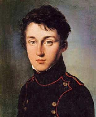
Sadi Carnot (1796 – 1832) (Mendoza, 2016), a French physicist and engineer was very interested in the improvement of steam engines to perform the tasks needed by modern society.
To simplify his analysis of the inner workings of an engine, Carnot devised a useful construct for examining what affect engine efficiency. His construct is the heat engine. The idea behind a heat engine is that it will take energy in the form of heat, and transform it into an equivalent amount of work.
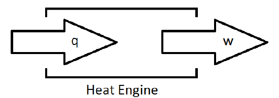
Unfortunately, such a device is impractical. As it turns out, nature prevents the complete conversion of energy into work with perfect efficiency. This leads to an important statement of the Second Law of Thermodynamics.
It is impossible to convert heat into an equivalent amount of work without some other changes occurring in the universe.
As such, a more reasonable picture of the heat engine is one which will allow for losses of energy to the surroundings.
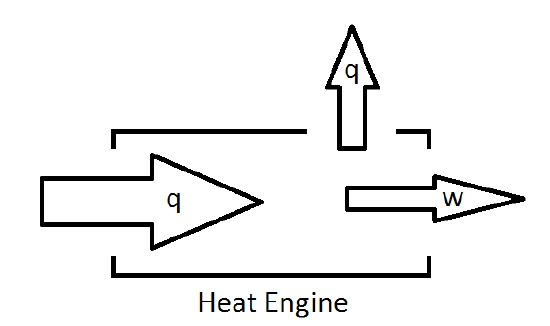
The fraction of energy supplied to the engine that can be converted to work defines the efficiency of the engine.
The Carnot Cycle
The Carnot cycle is a theoretical cyclic heat engine that can used to examine what is possible for an engine for which the job is convert heat into work. For simplicity, all energy provided to the engine occurs isothermally (and reversibly) at a temperature \(T_h\) and all of the energy lost to the surroundings also occurs isothermally and reversibly at temperature \(T_l\). In order to insure this, the system must change between the two temperatures adiabatically.
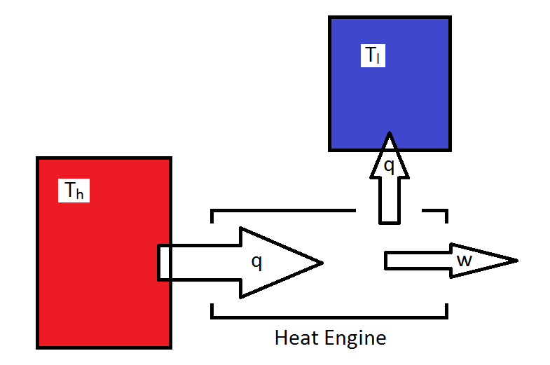
Thus, the cycle consists of four reversible legs, two of which are isothermal, and two of which are adiabatic.
- Isothermal expansion from p1 and V1 to p2 and V2 at Th.
- Adiabatic expansion from p2, V2, Th to p3, V3, Tl.
- Isothermal compression from p3 and V3 to p4 and V4 at Tl.
- Adiabatic compression from p4, V4, Tl to p1, V1, Th.
Plotted on a pressure-volume diagram, the Carnot cycle looks as follows:
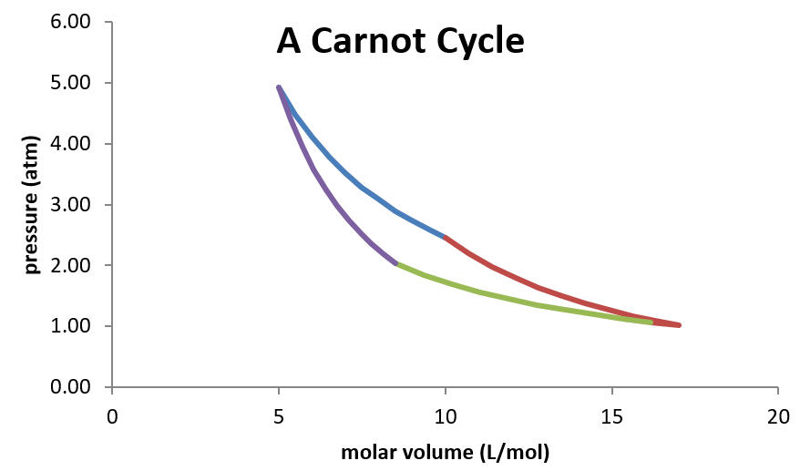
Because this is a closed cycle (the ending state is identical initial state) any state function must have a net change of zero as the system moves around the cycle. Furthermore, the efficiency of the engine can be expressed by the net amount of work the engine produces per unit of heat supplied to power the engine.
\[\epsilon = \dfrac{w_{net}}{q_h} \nonumber \]
In order to examine this expression, it is useful to write down expressions fo the heat and work flow in each of the four legs of the engine cycle.
| Leg | Heat | Work |
|---|---|---|
| I | qh = -nRTh ln(V2/V1) | nRTh ln(V2/V1) |
| II | 0 | CV(Tl – Th) |
| III | ql = -nRTl ln(V4/V3) | nRTl ln(V4/V3) |
| IV | 0 | CV(Th – Tl) |
The total amount of work done is given by the sum of terms in the thirst column. Clearly the terms for the two adiabatic legs cancel (as they have the same magnitude, but opposite signs.) So the total work done is given by
\[ w_{tot} = nRT_h \ln \left( \dfrac{V_2}{V_1} \right) + nRT_l \ln \left( \dfrac{V_4}{V_3} \right) \nonumber \]
The efficiency of the engine can be defined as the total work produced per unit of energy provided by the high temperature reservoir.
\[\epsilon = \dfrac{w_{tot}}{q_h} \nonumber \]
or
\[\epsilon = \dfrac{ nRT_h \ln \left( \dfrac{V_2}{V_1} \right) + nRT_l \ln \left( \dfrac{V_4}{V_3} \right)}{nRT_h \ln \left( \dfrac{V_2}{V_1} \right) } \label{eff1} \]
That expression has a lot of variables, but it turns out that it can be simplified dramatically. It turns out that by the choice of pathways connecting the states places a very important restriction on the relative values of V1, V2, V3 and V4. To understand this, we must consider how the work of adiabatic expansion is related to the initial and final temperatures and volumes. In Chapter 3, it was shown that the initial and final temperatures and volumes of an adiabatic expansion are related by
\[V_iT_i^{C_V/R} = V_fT_f^{C_V/R} \nonumber \]
or
\[ \dfrac{V_i}{V_f} = \left( \dfrac{T_f}{T_i} \right)^{C_V/R} \nonumber \]
Using the adiabatic expansion and compression legs (II and IV), this requires that
\[\dfrac{V_2}{V_2} = \left( \dfrac{T_h}{T_l} \right)^{C_V/R} \nonumber \]
and
\[\dfrac{V_4}{V_1} = \left( \dfrac{T_l}{T_h} \right)^{C_V/R} \nonumber \]
Since the second terms are reciprocals of one another, the first terms must be as well!
\[ \dfrac{V_2}{V_2}=\dfrac{V_1}{V_4} \nonumber \]
A simple rearrangement shows that
\[ \dfrac{V_2}{V_1}=\dfrac{V_3}{V_4} \nonumber \]
This is very convenient! It is what allows for the simplification of the efficiency expression (Equation \ref{eff1}) becomes
\[\epsilon = \dfrac{ \cancel{nR}T_h \cancel{\ln \left( \dfrac{V_2}{V_1} \right)} + \cancel{nR}T_l \cancel{ \ln \left( \dfrac{V_2}{V_1} \right)}}{\cancel{nR}T_h \cancel{\ln \left( \dfrac{V_2}{V_1} \right)} } \nonumber \]
Canceling terms in the numerator and denominator yields
\[\epsilon = \dfrac{T_g-T_l}{T_h} \label{eff2} \]
This expression gives the maximum efficiency and depends only on the high and low temperatures!
Also, it should be noted that the heat engine can be run backwards. By providing work to the engine, it can be forces to draw heat from the low temperature reservoir and dissipate it into the high temperature reservoir. This is how a refrigerator or heat pump works. The limiting efficiency of such a device can also be calculated using the temperatures of the hot can cold reservoirs.
What is the maximum efficiency of a freezer set to keep ice cream at a cool -10 oC, which it is operating in a room that is 25oC? What is the minimum amount of energy needed to remove 1.0 J from the freezer and dissipate it into the room?
Solution
The efficiency is given by Equation \ref{eff2} and converting the temperatures to an absolute scale, the efficiency can be calculated as
\[\epsilon = \dfrac{298\,K - 263\,K}{298\,K} \nonumber \]
This value can be used in the following manner
\[energy_{transferred} = \epsilon (work_{required}) \nonumber \]
So
\[ 1.0 \,J = 0.1174(w) \nonumber \]
or
\[w = 8.5\, J \nonumber \]
It is interesting to note that any arbitrary closed cyclical process can be described as a sum of infinitesimally small Carnot cycles, and so all of the conclusions reached for the Carnot cycle apply to any cyclical process.
Contributors
Patrick E. Fleming (Department of Chemistry and Biochemistry; California State University, East Bay)


