
5.4: Characterizing Couplings in 2D Spectra
- Page ID
- 298978

One of the unique characteristics of 2D spectroscopy is the ability to characterize molecular couplings1. This allows one to understand microscopic relationships between different objects, and with knowledge of the interaction mechanism, determine the structure or reveal the dynamics of the system. To understand how 2D spectra report on molecular interactions, we will discuss the spectroscopy using a model for two coupled electronic or vibrational degrees of freedom. Since the 2D spectrum reports on the eigenstates of the coupled system, understanding the coupling between microscopic states requires a model for the eigenstates in the basis of the interacting coordinates of interest. Traditional linear spectroscopy does not provide enough constraints to uniquely determine these variables, but 2D spectroscopy provides this information through a characterization of two-quantum eigenstates.
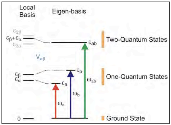
Since it takes less energy to excite one coordinate if a coupled coordinate already has energy in it, a characterization of the energy of the combination mode with one quantum of excitation in each coordinate provides a route to obtaining the coupling. This principle lies behind the use of overtone and combination band molecular spectroscopy to unravel anharmonic couplings.
The language for the different variables for the Hamiltonian of two coupled coordinates varies considerably by discipline. A variety of terms that are used are summarized below. We will use the underlined terms.
| System Hamiltonian \(H_S\) | Local or site basis (i,j) | Eigenbasis (a,b) | One-Quantum Eigenstates | Two-Quantum Eigenstates |
|---|---|---|---|---|
|
Local mode Hamiltonian Exciton Hamiltonian |
Sites Local modes |
Eigenstates Exciton states Delocalized states |
Fundamental v=0-1 |
Combination mode or band Overtone |
The model for two coupled coordinates can take many forms. We will pay particular attention to a Hamiltonian that describes the coupling between two local vibrational modes i and j coupled through a bilinear interaction of strength J:
\[\begin{aligned} H_{vib} &= H_i+H_j+V_{i,j} \\ &=\frac{p_i^2}{2m_i}+V(q_i)+\frac{p_j^2}{2m_j}+V(q_j)+Jq_iq_j \end{aligned} \label{9.1}\]
An alternate form cast in the ladder operators for vibrational or electronic states is the Frenkel exciton Hamiltonian
\[H_{vib,harmonic}\approx\hbar\omega_i\left(a_i^\dagger a_i\right)+\hbar\omega_j\left(a_j^\dagger a_j\right)+J\left(a_i^\dagger a_j+a_i a_j^\dagger\right) \label{9.2}\]
\[H_{elec}=E_ia_i^\dagger a_i+E_ja_j^\dagger a_j+\left(J_{ij}a_i^\dagger a_j+c.c\right) \label{9.3}\]
The bi-linear interaction is the simplest form by which the energy of one state depends on the other. One can think of it as the leading term in the expansion of the coupling between the two local states. Higher order expansion terms are used in another common form, the cubic anharmonic coupling between normal modes of vibration
\[H_{vib}=\left(\frac{p_i^2}{2m_i}+\frac{1}{2}k_iq_i^2+\frac{1}{6}g_{iii}q_i^2\right)+\left(\frac{p_j^2}{2m_j}+\frac{1}{2}k_jq_j^2+\frac{1}{6}g_{jjj}q_j^2\right)+\left(\frac{1}{2}g_{iij}q_i^2q_j+\frac{1}{2}g_{ijj}q_iq_j^2\right) \label{9.4}\]
In the case of eq. (9.2), the eigenstates and energy eigenvalues for the one-quantum states are obtained by diagonalizing the 2x2 matrix
\[H_S^{(1)}=\begin{pmatrix} E_{i=1} & J \\ J & E_{j=1} \end{pmatrix} \label{9.5}\]
\(E_{i=1}\) and \(E_{j=1}\) are the one-quantum energies for the local modes \(q_i\) and \(q_j\). These give the system energy eigenvalues
\[E_{a/b}=\Delta E \pm\left(\Delta E^2+J^2\right)^{1/2} \label{9.6}\]
\[\Delta E=\frac{1}{2}\left(E_{i=1}-E_{j=1}\right) \label{9.7}\]
\(E_a\) and \(E_b\) can be observed in the linear spectrum, but are not sufficient to unravel the three variables (site energies \(E_iE_j\) and coupling J) relevant to the Hamiltonian; more information is needed.
For the purposes of 2D spectroscopy, the coupling is encoded in the two-quantum eigenstates. Since it takes less energy to excite a vibration \(|i\rangle\) if a coupled mode \(|j\rangle\) already has energy, we can characterized the strength of interaction from the system eigenstates by determining the energy of the combination mode \(E_{ab}\) relative to the sum of the fundamentals:
\[\Delta_{ab}=E_a+E_b-E_{ab} \label{9.8}\]
In essence, with a characterization of \(E_{ab},E_a,E_b\) one has three variables that constrain \(E_i,E_j,J\). The relationship between \(\Delta_{ab}\) and J depends on the model.
Working specifically with the vibrational Hamiltonian eq. (9.1), there are three twoquantum states that must be considered. Expressed as product states in the two local modes these are \(|i,j\rangle = |20\rangle, |02\rangle,\) and \(|11\rangle\). The two-quantum energy eigenvalues of the system are obtained by diagonalizing the 3x3 matrix
\[ H_S^{(2)}=\begin{pmatrix} E_{i=2} & 0 & \sqrt{2}J \\ 0 & E_{j=2} & \sqrt{2}J \\ \sqrt{2}J & \sqrt{2}J & E_{i=1}+E_{j=1} \end{pmatrix} \label{9.9}\]
Here \(E_{i=2}\) and \(E_{j=2}\) are the two-quantum energies for the local modes \(q_i\) and \(q_j\). These are commonly expressed in terms of \(\delta E_i\), the anharmonic shift of the i=1-2 energy gap relative to the i=0-1 one-quantum energy:
\[\begin{aligned} \delta E_i &= \left(E_{i=1}-E_{i=0}\right)-\left(E_{i=2}-E_{i=1}\right) \\ \delta\omega_i &= \omega_{10}^i-\omega_{21}^i \end{aligned} \label{9.10}\]
Although there are analytical solutions to eq. (9.9), it is more informative to examine solutions in two limits. In the strong coupling limit (\(J\lt\lt\Delta E\)), one finds
\[\Delta_{ab}=J \label{9.11}\]
For vibrations with the same anharmonicity \(\delta E\) with weak coupling between them (\(J\lt\lt\Delta E\)), perturbation theory yields
\[\Delta_{a b}=\delta E \frac{J^{2}}{\Delta E^{2}} \label{9.12}\]
This result is similar to the perturbative solution for weakly coupled oscillators of the form given by eq. (9.4)
\[\Delta_{a b}=g_{i i j}^{2}\left(\frac{4 E_{i}}{E_{j}^{2}-4 E_{i}^{2}}\right)+g_{i j j}^{2}\left(\frac{4 E_{j}}{E_{i}^{2}-4 E_{j}^{2}}\right) \label{9.13}\]
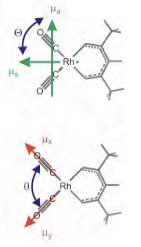
Example \(\PageIndex{1}\): \(\ce{Rh(CO)2(acac)}\)
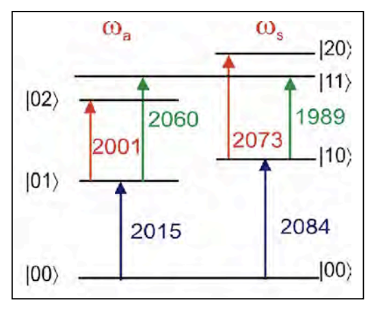
So, how do these variables present themselves in 2D spectra? Here it is helpful to use a specific example: the strongly coupled carbonyl vibrations of \(\ce{Rh(CO)2(acac)}\) or RDC. For the purpose of 2D spectroscopy with infrared fields resonant with the carbonyl transitions, there are six quantum states (counting the ground state) that must be considered. Coupling between the two degenerate CO stretches leads to symmetric and anti-symmetric one-quantum eigenstates, which are more commonly referred to by their normal mode designations: the symmetric and asymmetric stretching vibrations. For n=2 coupled vibrations, there are n(n−1)/2 = 3 two-quantum eigenstates. In the normal mode designation, these are the first overtones of the symmetric and asymmetric modes and the combination band. This leads to a six level system for the system eigenstates, which we designate by the number of quanta in the symmetric and asymmetric stretch: \(|00\rangle\), \(|s\rangle\) = \(|10\rangle\), \(|a\rangle\) = \(|01\rangle\), \(|2s\rangle\) = \(|20\rangle\), \(|2a\rangle\) = \(|02\rangle\), and \(|sa\rangle\) = \(|11\rangle\). For a model electronic system, there are four essential levels that need to be considered, since Fermi statistics does not allow two electrons in the same state: \(|00\rangle\), \(|10\rangle\), \(|01\rangle\), and \(|11\rangle\).
We now calculate the nonlinear third-order response for this six-level system, assuming that all of the population is initially in the ground state. To describe a double-resonance or Fourier transform 2D correlation spectrum in the variables \(\omega_1\) and \(\omega_3\), include all terms relevant to pump-probe experiments: \(-k_1 +k_2 +k_3\) (\(S_{I}\), rephasing) and \(k_1 - k_2 +k_3\) (\(S_{II}\), non-rephasing). After summing over many interaction permutations using the phenomenological propagator, keeping only dipole allowed transitions with ±1 quantum, we find that we expect eight resonances in a 2D spectrum. For the case of the rephasing spectrum \(S_I\)
\[\begin{aligned} S_I(\omega_1,\omega_3) &= \frac{2|\mu_{s,0}|^4}{\left[i(\omega_1+\omega_{s,0})+\Gamma_{s,0}\right]\left[i(\omega_3-\omega_{s,0})+\Gamma_{s,0}\right]} + \frac{2|\mu_{a,0}|^4}{\left[i(\omega_1+\omega_{a,0})+\Gamma_{a,0}\right]\left[i(\omega_3-\omega_{a,0})+\Gamma_{a,0}\right]} \\ &+ \frac{2|\mu_{a,0}|^2|\mu_{s,0}|^2}{\left[i(\omega_1+\omega_{s,0})+\Gamma_{s,0}\right]\left[i(\omega_3-\omega_{a,0})+\Gamma_{a,0}\right]} + \frac{2|\mu_{a,0}|^2|\mu_{s,0}|^2}{\left[i(\omega_1+\omega_{a,0})+\Gamma_{a,0}\right]\left[i(\omega_3-\omega_{s,0})+\Gamma_{b,0}\right]} \\ &- \frac{|\mu_{s,0}|^2|\mu_{2s,s}|^2}{\left[i(\omega_1+\omega_{s,0})+\Gamma_{s,0}\right]\left[i(\omega_3-\omega_{s,0}+\Delta_{s})+\Gamma_{2s,s}\right]} - \frac{|\mu_{a,0}|^2|\mu_{2a,a}|^2}{\left[i(\omega_1+\omega_{a,0})+\Gamma_{a,0}\right]\left[i(\omega_3-\omega_{a,0}+\Delta_{a})+\Gamma_{2a,a}\right]} \\ &-\frac{|\mu_{s,0}|^2|\mu_{as,s}|^2+\mu_{0,s}\mu_{a,0}\mu_{as,a}\mu_{s,as}}{\left[i(\omega_1+\omega_{s,0})+\Gamma_{s,0}\right]\left[i(\omega_3-\omega_{a,0}+\Delta_{as})+\Gamma_{as,s}\right]} - \frac{|\mu_{a,0}|^2|\mu_{as,a}|^2+\mu_{0,a}\mu_{s,0}\mu_{as,s}\mu_{a,as}}{\left[i(\omega_1+\omega_{a,0})+\Gamma_{a,0}\right]\left[i(\omega_3-\omega_{s,0}+\Delta_{as})+\Gamma_{as,a}\right]} \\ &\equiv {\bf 1+1'+2+2'+3+3'+4+4'} \end{aligned} \label{9.14}\]
To discuss these peaks we examine how they appear in the experimental Fourier transform 2D IR spectrum of RDC, here plotted both as in differential absorption mode and absolute value mode. We note that there are eight peaks, labeled according to the terms i eq. (9.14) from which they arise. Each peak specifies a sequence of interactions with the system eigenstates, with excitation at a particular \(\omega_1\) and detection at given \(\omega_3\). Notice that in the excitation dimension \(ω_1\) all of the peaks lie on one of the fundamental frequencies. Along the detection axis \(\omega_3\) resonances are seen at all six one-quantum transitions present in our system.
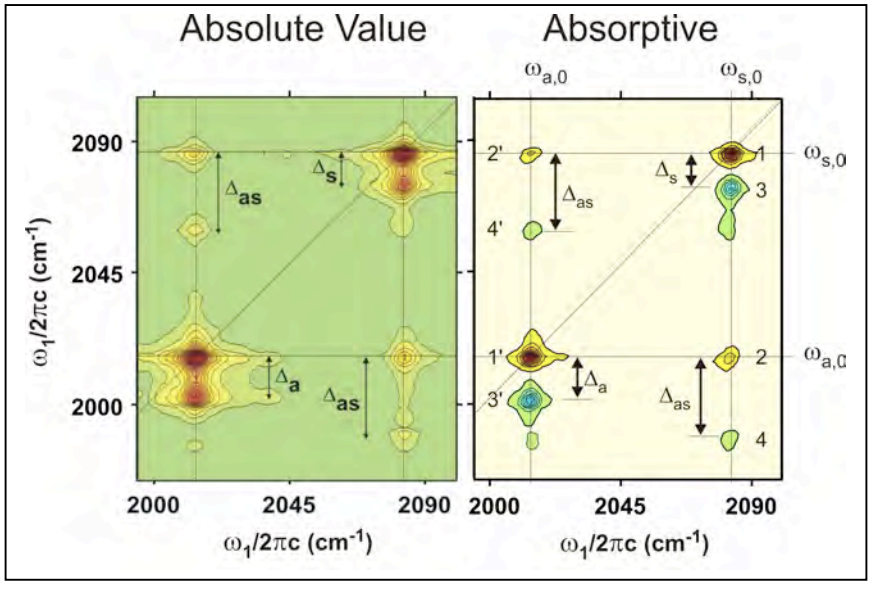
More precisely, there are four features: two diagonal and two cross peaks each of which are split into a pair. The positive diagonal and cross peak features represent evolution on the fundamental transitions, while the split negative features arise from propagation in the two-quantum manifold. The diagonal peaks represent a sequence of interactions with the field that leaves the coherence on the same transition during both periods, where as the split peak represents promotion from the fundamental to the overtone during detection. The overtone is anharmonically shifted, and therefore the splitting between the peaks, ,\(\Delta_a,\Delta_s\), gives the diagonal anharmonicity. The cross peaks arise from the transfer of excitation from one fundamental to the other, while the shifted peak represents promotion to the combination band for detection. The combination band is shifted in frequency due to coupling between the two modes, and therefore the splitting between the peaks in the off-diagonal features \(\Delta_{as}\) gives the off-diagonal anharmonicity.
Notice for each split pair of peaks, that in the limit that the anharmonicity vanishes, the two peaks in each feature would overlap. Given that they have opposite sign, the peaks would destructively interfere and vanish for a harmonic system. This is a manifestation of the rule that a nonlinear response vanishes for a harmonic system. So, in fact, a 2D spectrum will have signatures of whatever types of vibrational interactions lead to imperfect interference between these two contributions. Nonlinearity of the transition dipole moment will lead to imperfect cancellation of the peaks at the amplitude level, and nonlinear coupling with a bath will lead to different lineshapes for the two features.
With an assignment of the peaks in the spectrum, one has mapped out the energies of the one- and two-quantum system eigenstates. These eigenvalues act to constrain any model that will be used to interpret the system. One can now evaluate how models for the coupled vibrations match the data. For instance, when fitting the RDC spectrum to the Hamiltonian in eq. (9.1) for two coupled anharmonic local modes with a potential of the form \(V\left(q_{i}\right)=\frac{1}{2} k_{i} q_{i}^{2}+\frac{1}{6} g_{i i i} q_{i}^{3}\), we obtain \(\hbar \omega_{10}^{i}=\hbar \omega_{10}^{j}=2074 \mathrm{~cm}^{-1}\), \(J_{i j}=35 \mathrm{~cm}^{-1}\), and \(g_{iii} = g_{jjj} = 172 \mathrm{~cm}^{-1}\). Alternatively, we can describe the spectrum through eq. (9.4) as symmetric and asymmetric normal modes with diagonal and off-diagonal anharmonicity. This leads to \(\hbar \omega_{10}^{a}=2038 \mathrm{~cm}^{-1}\), \(\hbar \omega_{10}^{s}=2108 \mathrm{~cm}^{-1}\), \(g_{a a a}=g_{s s s}=32 \mathrm{~cm}^{-1}\), and \(g_{s s a}=g_{a a s}=22 \mathrm{~cm}^{-1}\). Provided that one knows the origin of the coupling and its spatial or angular dependence, one can use these parameters to obtain a structure.
References
1. Khalil M, Tokmakoff A. “Signatures of vibrational interactions in coherent two-dimensional infrared spectroscopy.” Chem Phys. 2001;266(2-3):213-30; Khalil M, Demirdöven N, Tokmakoff A. “Coherent 2D IR Spectroscopy: Molecular structure and dynamics in solution.” J Phys Chem A. 2003;107(27):5258-79; Woutersen S, Hamm P. Nonlinear twodimensional vibrational spectroscopy of peptides. J Phys: Condens Mat. 2002;14:1035-62.