4.4: How Can you Characterize Fluctuations and Spectral Diffusion?

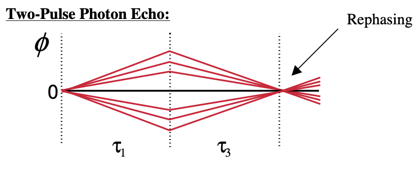
The rephasing ability of the photon echo experiment provides a way of characterizing memory of the energy gap transition frequency initially excited by the first pulse. For a static inhomogeneous lineshape, perfect memory of transition frequencies is retained through the experiment, whereas homogeneous broadening implies extremely rapid dephasing. So, let’s first examine the polarization for a two-pulse photon echo experiment on a system with homogeneous and inhomogeneous broadening by varying \(\Delta/\Gamma_{eg}\). Plotting the polarization as proportional to the response in eq. (5.3.7):

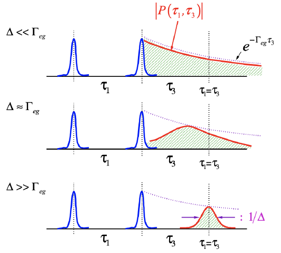
We see that following the third pulse, the polarization (red line) is damped during \(\tau_3\) through homogeneous dephasing at a rate \(\Gamma_{eg}\), regardless of Δ. However in the inhomogeneous case \(\Delta\gt\gt\Gamma_{eg}\), any inhomogeneity is rephased at \(\tau_1=\tau_3\). The shape of this echo is a Gaussian with width ~ 1/ Δ . The shape of the echo polarization is a competition between the homogeneous damping and the inhomogeneous rephasing.

Normally, one detects the integrated intensity of the radiated echo field. Setting the pulse delay \(\tau_1=\tau\),

\[S(\tau)\propto\int_0^{\infty}d\tau_3|P^{(3)}(\tau,\tau_3)|^2 \label{5.4.1}\]

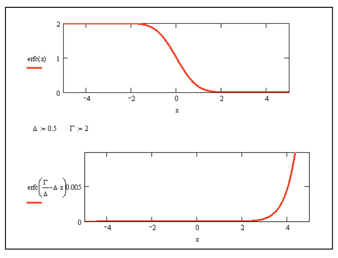
\[S(\tau)=exp\left(-4\Gamma_{eg}\tau-\frac{\Gamma_{eg}^2}{\Delta^2}\right)\cdot erfc\left(-\Delta\tau+\frac{\Gamma_{eg}}{\Delta}\right) \label{5.4.2}\]

where \(erfc(x)=1-erf(x)\) is the complementary error function. For the homogeneous and inhomogeneous limits of this expression we find

\[\Delta \lt\lt \Gamma_{eg} \Rightarrow S(\tau)\propto e^{-2\Gamma_{eg}\tau} \label{5.4.3}\]

\[\Delta \gt\gt \Gamma_{eg} \Rightarrow S(\tau)\propto e^{-4\Gamma_{eg}\tau} \label{5.4.4}\]

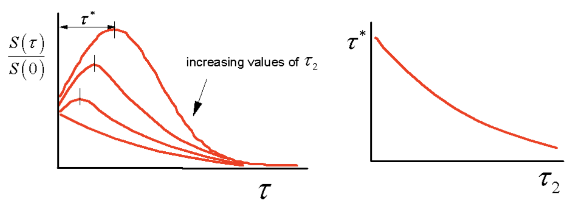
In either limit, the inhomogeneity is removed from the measured decay. In the intermediate case, we observe that the leading term in eq. (5.4.2) decays whereas the second term rises with time. This reflects the competition between homogeneous damping and the inhomogeneous rephasing. As a result, for the intermediate case \((\Delta \approx \Gamma_{ab})\) we find that the integrated signal \(S(\tau)\) has a maximum signal for \(\tau\gt 0\).

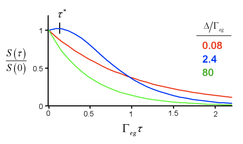
The delay of maximum signal, \(\tau^*\), is known as the peak shift. The observation of a peak shift is an indication that there is imperfect ability to rephrase. Homogenous dephasing, i.e. fluctuations fast on the time scale of \(\tau\), are acting to scramble memory of the phase of the coherence initially created by the first pulse.

In the same way, spectral diffusion (processes which randomly modulate the energy gap on time scales equal or longer than \(\tau\)) randomizes phase. It destroys the ability for an echo to form by rephasing. To characterize these processes through an energy gap correlation function, we can perform a three-pulse photon echo experiment. The three pulse experiment introduces a waiting time \(\tau_2\) between the two coherence periods, which acts to define a variable shutter speed for the experiment. The system evolves as a population during this period, and therefore there is nominally no phase acquired. We can illustrate this through a lens analogy:

Lens Analogy: For an inhomogeneous distribution of oscillators with different frequencies, we define the phase acquired during a time period through \(e^{i\phi}=e^{i(\delta\omega_i t)}\)

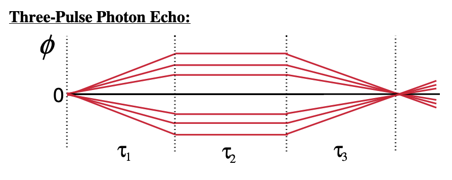
Since we are in a population state during \(\tau_2\), there is no evolution of phase. Now to this picture we can add spectral diffusion as a slower random modulation of the phase acquired during all time periods. If the system can spectrally diffuse during \(\tau_2\), this degrades the ability of the system to rephase and echo formation is diminished.

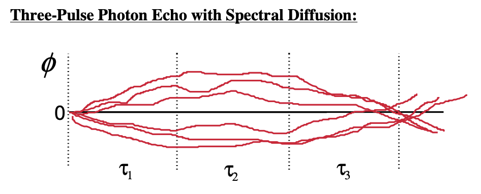
Since spectral diffusion destroys the rephasing, the system appears more and more “homogeneous” as \(\tau_2\) is incremented. Experimentally, one observes how the peak shift of the integrated echo changes with the waiting time \(\tau_2\). It will be observed to shift toward \(\tau^*=0\) as a function of \(\tau_2\).

In fact, one can show that the peak shift with \(\tau_2\) decays with a form given by the the correlation function for system-bath interactions:

\[\tau^*(\tau_2)\propto C_{eg}(\tau) \label{5.4.5}\]

Using the lineshape function for the stochastic model \(g(t)=\Delta^2\tau_c^2\left[exp(-t/\tau_c)+t/\tau_c-1\right]\), you can see that for times \(\tau_2\gt\tau_c\),

\[\tau^*(\tau_2)\propto exp(-\tau_2/\tau_c)\Rightarrow \left\langle\delta\omega_{eg}(\tau)\delta\omega_{eg}(0)\right\rangle \label{5.4.6}\]

Thus echo peak shift measurements are a general method to determine the form to \(C_{eg}(\tau)\) or \(C_{eg}''(\omega)\) or \(\rho(\omega)\). The measurement time scale is limited only by the population lifetime.