3.2: Navier-Stokes Hydrodynamic Equations

Basic Equations

Conservation of Mass

Consider a fixed volume in space, such as that pictured in Figure \(3.6\)

The total number of particles in the region at any point in time can be found by taking the sum over the density at all points:

\[N=\int_{V} \rho(\vec{r}) d \vec{r}\]

The change in \(N\) over time depends upon the flux, which can be found by integration over a surface or a volume

\[\frac{d N}{d t}=J_{i n}-J_{o u t}=-\oint_{\partial V} \vec{J} \cdot d \vec{S}=-\int \vec{\nabla} \cdot \vec{J} d V\]

We can rewrite the change in the number of particles in terms of density:

\[\frac{d N}{d t}=\int \frac{d \rho}{d t} d \vec{r}=-\int \vec{\nabla} \cdot \vec{J} d V\]

Remove the spacial integration and rearrange

\[\frac{d \rho}{d t}+\vec{\nabla} \cdot \vec{J}=0\]

To express the equation in terms of density and velocity, we rewrite the flux as \(\vec{J}=\rho \vec{v}\), so that

\[\nabla \vec{J}=\vec{\nabla} \cdot(\rho \vec{v})\]

Then the conservation of mass is given by:

Figure 3.6: The flow of material into and out of a fixed region of space

Continuity Equations In general, for any dynamic quantity \(A\), we can define a density \(\rho\) and write down a continuity equation.

This equation will be determined by the interaction between currents \(\vec{J}\) and sources \(\sigma\).

\[\frac{\partial \rho A}{\partial t}+\vec{\nabla} \cdot \vec{J}=\sigma\]

The total current \(\vec{J}\) can be modelled as the sum of a conservative term \(\vec{J}_{V}=\rho A \vec{v}\) and a dissipative term \(\vec{J}_{D}\).

\[\vec{J}=\vec{J}_{V}+\vec{J}_{D}\]

The source \(\sigma\) can be written as the sum of external sources \(\sigma_{\text {ext }}\) and production sources \(\sigma_{D}\)

\[\sigma=\sigma_{\text {ext }}+\sigma_{D}\]

Therefore, the continuity equation for \(A\) can be written more explicitly as

\[\frac{\partial \rho A}{\partial t}+\vec{\nabla} \cdot(\rho A \vec{v})+\vec{\nabla} \cdot \vec{J}_{D}=\sigma_{e x t}+\sigma_{D}\]

In the physical world there are five conserved quantities: the density, the momentum (in three directions), and the energy (or entropy).

\[A=\{1, m \vec{v}, S\}\]

Therefore, we will find five continuity equations. We have already found the continuity equation for density, and in the next two sections we will find the equations for momentum and entropy.

Figure 3.7: The flow and forces for a dynamic quantity

Momentum Equation (Navier-Stokes equations)

To find the continuity equation for momentum, substitute \(A=m \vec{v}\) into the general continuity equation.

\[\frac{\partial \rho m \vec{v}}{\partial t}+\vec{\nabla} \cdot(\rho m \vec{v}: \vec{v})+\vec{\nabla} \cdot \overrightarrow{\vec{J}}_{D}=\vec{\sigma}_{e x t}+\vec{\sigma}_{D}\]

We assume that the production force is zero. The external force is pressure, which acts to create a net momentum or acceleration.

\[\vec{\sigma}_{\text {ext }}=\rho \vec{F}-\vec{\nabla} P\]

The terms representing conservative and dissipative current are both tensors. This is because momentum is a vector, and so the current, which represents the change in momentum, must be a tensor. The conservative current is given by

\[\overrightarrow{\vec{J}}_{V}=(\rho m \vec{v}: \vec{v})\]

The dissipative current is the stress tensor \(\overrightarrow{\vec{J}}_{D}=-\overrightarrow{\vec{\Pi}}\). The continuity equation for momentum can then be written as

\[m \frac{\partial \rho \vec{v}}{\partial t}+\vec{\nabla} \cdot(\rho m \vec{v}: \vec{v})+\vec{\nabla} P=\rho \vec{F}+\vec{\nabla} \cdot \overrightarrow{\vec{\Pi}}\]

Let’s take a closer look at the stress tensor. For an isotropic medium, the stress tensor can be expressed as

\[\Pi_{i, j}=\eta_{B}(\vec{\nabla} \cdot \vec{v}) \delta_{i, j}+\eta\left(\partial_{i} v_{j}+\partial_{j} v_{i}-\frac{2}{3}(\vec{\nabla} \cdot \vec{v}) \delta_{i, j}\right)\]

where \(\eta_{B}\) is the bulk viscosity. It gives the expected change in volume resulting from an applied stress. Likewise, \(\eta\) is the shear viscosity. This gives the expected amount of shearing, or change in shape, resulting from an applied stress. The final term \(\partial_{i} v_{j}+\partial_{j} v_{i}-\frac{2}{3} \nabla \vec{v} \delta_{i, j}\) is a traceless symmetric component which changes the shape, but not the volume, of the medium.

We can express the change in the stress tensor as

\[(\vec{\nabla} \cdot \overrightarrow{\mathrm{\Pi}})_{i}=\sum_{j} \nabla_{j} \Pi_{j, i}=\left(\frac{1}{3} \eta+\eta_{B}\right) \nabla_{i}(\vec{\nabla} \cdot \vec{v})+\eta \nabla^{2} v_{i}\]

With this, we can rewrite the momentum continuity equation as

\[m \frac{\partial \rho \vec{v}}{\partial t}+\vec{\nabla} \cdot(\rho m \vec{v}: \vec{v})+\vec{\nabla} P=\left(\frac{1}{3} \eta+\eta_{B}\right) \vec{\nabla}(\vec{\nabla} \cdot \vec{v})+\eta \nabla^{2} \vec{v}\]

This is also called the Navier-Stokes equation.

Entropy Equation (heat-diffusion)

To find the continuity equation for entropy, substitute \(A=s\) in to the general continuity equation. In this case, we are thinking of the entropy for each particle and not the entire system, so a lowercase \(s\) is used.

\[\frac{\partial \rho s}{\partial t}+\vec{\nabla} \cdot(\rho s \vec{v})+\vec{\nabla} \cdot \vec{J}_{D}=\sigma_{e x t}+\sigma_{D}\]

We can simplify this expression by assuming that there are no forces that that create or destroy entropy, so \(\sigma_{\text {ext }}+\sigma_{D}=0\) We also know that entropy flows from high temperatures to low temperatures, so

\[\vec{J}_{D} \propto-\vec{\nabla} \cdot \vec{T}\]

Write this explicitly using the constant \(\lambda\)

\[\vec{J}_{D}=-\frac{\lambda \vec{\nabla} T}{T}\]

Then, substitute this to get the continuity equation

\[\frac{\partial \rho s}{\partial t}+\vec{\nabla} \cdot(\rho s \vec{v})-\lambda \vec{\nabla} \cdot\left(\frac{\vec{\nabla} T}{T}\right)=0\]

We now have expressions for the 5 continuity equations for number of particles, momentum, and energy.

\[\begin{aligned} \frac{d \rho}{d t}+\vec{\nabla} \cdot(\rho \vec{v}) &=0 \\ m \frac{\partial \rho \vec{v}}{\partial t}+\vec{\nabla} \cdot(\rho m \vec{v}: \vec{v})+\vec{\nabla} P &=\vec{\nabla} \cdot \overrightarrow{\vec{\Pi}} \\ \frac{\partial \rho s}{\partial t}+\vec{\nabla} \cdot(\rho s \vec{v})-\lambda \vec{\nabla} \cdot\left(\frac{\vec{\nabla} T}{T}\right) &=0 \end{aligned}\]

The solution to this set of equations gives \(\rho(k, t)\). Though it is impossible to solve analytically, approximate solutions can be obtained by linearizing the equations.

Linearized Hydrodynamic Equations

The hydrodynamic equations are impossible to solve analytically. However, it is possible to obtain approximate solutions by linearizing the equations. Define the operator

\[\mathcal{L}(A)=\frac{\partial A}{\partial t}\]

For a time-independent quantity \(A_{S}\),

\[\mathcal{L}\left(A_{S}\right)=\frac{\partial A_{S}}{\partial t}=0\]

We can construct any quantity \(A\) as the sum of a time-independent, "stable" part \(A_{S}\) and a fluctuating part \(\delta A\)

\[A=A_{S}+\delta A\]

Then we can write \(\mathcal{L}(A)\) as an expansion. If we truncate the expansion at the first order, linear term, we find that

\[\mathcal{L}(A)=\mathcal{L}\left(A_{S}+\delta A\right)=\mathcal{L}\left(A_{S}\right)+\mathcal{L}(\delta A)=\frac{\partial \delta A}{\partial t}\]

For a homogeneous solution, \(\rho\) is a constant. There is no collective kinetic motion, only small Boltzmann motions which average to zero. Therefore, \(\overrightarrow{v_{o}}=0\). Entropy is also a constant. Therefore, we have three constants:

\[\rho_{o}, \overrightarrow{v_{o}}=0, S_{o}\]

Since the density, velocity, and entropy are constants for a homogeneous solution, we can construct these quantities for a non-homogeneous solution by expanding around them:

\[\begin{aligned} \rho=\rho_{o}+\delta \rho \\ S=S_{o}+\delta S \\ \vec{v} \end{aligned}\]

We can also expand around a constant temperature and pressure:

\[\begin{aligned} &T=T_{o}+\delta T \\ &P=P_{o}+\delta P \end{aligned}\]

Start by substituting the density expansion into the density continuity equation

\[\begin{aligned} \frac{d}{d t}\left(\rho_{o}+\delta \rho\right)+\vec{\nabla} \cdot\left[\left(\rho_{o}+\delta \rho\right) \vec{v}\right]=0 \\ \frac{d \delta \rho}{d t}+\vec{\nabla} \cdot\left(\rho_{o} \vec{v}\right)=0 \end{aligned}\]

This is the linearized number density continuity equation. To reach the final expression, we have used that \(\frac{d \rho_{o}}{d t}=0\). We have also ignored the term \(\vec{\nabla} \cdot(\delta \rho \vec{v})\) because it is of quadratic order and we can assume that it is negligible. In order to linearize the continuity equation for entropy, begin by expanding the original expression.

\[\rho \frac{\partial \delta s}{\partial t}+s_{o} \frac{\partial \rho}{\partial t}+s_{o} \vec{\nabla} \cdot(\rho \vec{v})+\rho \vec{\nabla} \cdot(\delta s \vec{v})-\lambda \vec{\nabla} \cdot\left(\frac{\vec{\nabla} T}{T}\right)=0\]

The second and third term can be combined and will go to zero by conservation of mass. The fourth term is negligible. Then by substituting in the expansions and keeping only the linear terms, the expression simplifies to:

\[\rho_{o} \frac{\partial \delta s}{\partial t}-\frac{\lambda}{T_{o}} \nabla^{2} \delta T=0\]

Similarly we can linearize the momentum continuity equation, the solution is

\[m \rho_{o} \frac{\partial \vec{v}}{\partial t}+\vec{\nabla} \delta P=\left(\frac{1}{3} \eta+\eta_{B}\right)(\vec{\nabla}: \vec{\nabla}) \cdot \vec{v}+\eta \nabla^{2} \vec{v}\]

In summary, the linearized hydrodynamic equations are given by

\[\begin{aligned} \frac{d \delta \rho}{d t}+\rho_{o} \vec{\nabla} \cdot \vec{v} &=0 \\ m \rho_{o} \frac{\partial \vec{v}}{\partial t}+\nabla \delta P &=\left(\frac{1}{3} \eta+\eta_{B}\right)(\vec{\nabla}: \vec{\nabla}) \cdot \vec{v}+\eta \nabla^{2} \vec{v} \\ \rho_{o} \frac{\partial \delta s}{\partial t}-\frac{\lambda}{T_{o}} \nabla^{2} \delta T &=0 \end{aligned}\]

Transverse Hydrodynamic Modes

In order to solve the eigenvalue equation, we need to decompose the velocity into its transverse and longitudinal components. Begin by rewriting the velocity in terms of its Fourier components

\[\vec{v}(r, t)=\frac{1}{(2 \pi)^{3}} \int \vec{v}(k, t) e^{i \vec{k} \cdot \vec{r}} d \vec{k}\]

Through substitution, the momentum continuity equation becomes

\[m \rho_{o} \frac{\partial \overrightarrow{v_{k}}}{\partial t}+i \vec{k} P_{k}=\left(\frac{1}{3} \eta+\eta_{B}\right)(i \vec{k})\left(i \vec{k} \cdot \overrightarrow{v_{k}}\right)+\eta(\vec{k})^{2} \overrightarrow{v_{k}}\]

Now, decompose \(\vec{v}(k, t)\) into its 3 components

\[v(k, t)=v_{x k}(t) \hat{x}+v_{y k}(t) \hat{y}+v_{z k}(t) \hat{z}\]

A longitudinal mode is one in which the velocity vector points parallel to the \(\vec{k}\) vector, and a transverse mode is one in which the velocity vector points perpendicular to the \(\vec{k}\) vector. We can decide arbitrarily that the \(\vec{k}\) vector points in the \(z\) direction. Therefore, \(v_{z k}(t)\) is the longitudinal current and \(v_{x k}(t)\) and \(v_{y k}(t)\) are the transverse currents.

Figure 3.8: Velocity components in k-space

which is easy to solve, yielding the solution

\[v_{T k}(t)=v_{T k}(0) e^{-\gamma_{T} k^{2} t}\]

where \(\gamma_{T}=\frac{\eta}{m \rho_{o}}\) is the kinematic shear viscosity.

This result looks like a diffusion equation

\[\frac{\partial P_{k}}{\partial t}=-D k^{2} P_{k}\]

Therefore, \(\gamma_{T}\) can be interpreted as diffusion constant for velocity.

Longitudinal Hydrodynamic modes

Solving the Continuity Equations

It is much more difficult to solve for the longitudinal velocity component of the current because not as many terms go to zero.

Fourier Transform of the density Begin by writing the density in terms of its Fourier components

\[\vec{\rho}(r, t)=\frac{1}{(2 \pi)^{3}} \int \vec{\rho}(k, t) e^{i \vec{k} \vec{r}} d \vec{k}\]

Using this expression, the linearized hydrodynamic equations can be written in terms of the Fourier components of the density. Note that hereafter, for brevity, we will drop the \(\delta\) signs of the transformed variables. Readers should keep in mind that these \(k\)-space variables always refer to the Fourier transform of the fluctuations away from equilibrium.

\[\begin{aligned} \frac{d \rho_{k}}{d t}+i k \rho_{o} v_{k} &=0 \\ m \rho_{o} \frac{\partial v_{k}}{\partial t}+i k P_{k}+\left(\frac{4}{3} \eta+\eta_{B}\right) k^{2} v_{k} &=0 \\ \rho_{o} \frac{\partial s_{k}}{\partial t}+\frac{\lambda}{T_{o}} k^{2} T_{k} &=0 \end{aligned}\]

Also we denote the velocity as \(v_{k}\) for simplicity. However, it is important to remember that this only refers to the longitudinal velocity, \(v_{z, k}\). Choosing independent variables As written, the three continuity equations have five variables: \(\rho_{k}, v_{k}, T_{k}, P_{k}\), and \(S_{k}\). Luckily, these variables are not all independent. Let \(\rho_{k}, v_{k}\), and \(T_{k}\) be the three independent variables. We can use thermodynamic relations to rewrite \(P_{k}\) and \(S_{k}\) in terms of these variables.

The Helmholtz free energy is a function of temperature and density, \(F(T, \rho)\). We can write this in differential form:

\[d F=-S d T+P d \rho\]

This is a total differential of the form:

\[d z=\left(\frac{\partial z}{\partial x}\right)_{y} d x+\left(\frac{\partial z}{\partial y}\right)_{x} d y\]

Using this, we can write the entropy \(S\) and the pressure \(P\) in differential form

\[\begin{aligned} S=-\left(\frac{\partial F}{\partial T}\right)_{\rho} \\ P=\left(\frac{\partial F}{\partial \rho}\right)_{T} \end{aligned}\]

Define the variable \(\alpha\) as

\[\alpha=\left(\frac{\partial P}{\partial T}\right)_{\rho}=\frac{\partial}{\partial T}\left(\frac{\partial F}{\partial \rho}\right)_{T}=\frac{\partial}{\partial \rho}\left(\frac{\partial F}{\partial T}\right)_{\rho}=-\left(\frac{\partial S}{\partial \rho}\right)_{T}\]

Here we have used the property that for continuous functions, the mixed partial second derivatives are equal. This gives one of the Maxwell relations.

We will also use a couple of well known relations, the isothermal speed of sound:

\[c_{T}=\sqrt{\frac{1}{m}\left(\frac{\partial P}{\partial \rho}\right)_{T}}\]

and the specific heat:

\[C_{V}=T\left(\frac{\partial S}{\partial T}\right)_{\rho}\]

With these relations in hand, we can rewrite the pressure \(P\) and the entropy \(S\) in terms of temperature \(T\) and density \(\rho\) :

\[\begin{aligned} d P=\left(\frac{\partial P}{\partial \rho}\right)_{T} d \rho+\left(\frac{\partial P}{\partial T}\right)_{\rho} d T=m C_{T}^{2} d \rho+\alpha d T \\ T_{o} d S=T_{o}\left(\frac{\partial S}{\partial \rho}\right)_{T} d \rho+T_{o}\left(\frac{\partial S}{\partial T}\right)_{\rho} d T=-T_{o} \alpha d \rho+C_{V} d T \end{aligned}\]

The Condensed Equations With these substitutions, we can rewrite the continuity equations in terms of the independent variables \(\rho_{k}, v_{k}\), and \(T_{k}\).

\[\begin{aligned} \frac{d \rho_{k}}{d t}+i k \rho_{o} v_{k} &=0 \\ \dot{v}_{k}+\frac{i k}{m \rho_{o}}\left[C_{T}^{2} m \rho_{k}+\alpha T_{k}\right]+b k^{2} v_{k} &=0 \\ \dot{T}_{k}+i k\left(\frac{T_{o} \alpha \rho_{o}}{C_{V}}\right) v_{k}+a k^{2} T_{k} &=0 \end{aligned}\]

where we have defined the constants \(a\) and \(b\)

\[\begin{aligned} a=\frac{\lambda}{\rho_{o} C_{V}} \\ b=\left(\eta_{B}+\frac{4}{3} \eta\right) \frac{1}{m \rho_{o}} \end{aligned}\]

and \(\rho_{k}=-i k \rho_{o} v_{k}\) is used to simplify the last equation.

The Laplace Transform To further simplify the equations, use the Laplace transform of each variable:

\[\begin{array}{llll} \hat{\rho}_{k}(z)=\int_{0}^{\infty} e^{-z t} \rho_{k}(t) d t & \text { and } & \rho_{k}(t)=\frac{1}{2 \pi i} \int_{\delta-i \infty}^{\delta+i \infty} e^{z t} \hat{\rho}_{k}(z) d z \\ \hat{v}_{k}(z)=\int_{0}^{\infty} e^{-z t} v_{k}(t) d t & \text { and } & v_{k}(t)=\frac{1}{2 \pi i} \int_{\delta-i \infty}^{\delta+i \infty} e^{z t} \hat{v}_{k}(z) d z \\ \hat{T}_{k}(z)=\int_{0}^{\infty} e^{-z t} T_{k}(t) d t \quad \text { and } & T_{k}(t)=\frac{1}{2 \pi i} \int_{\delta-i \infty}^{\delta+i \infty} e^{z t} \hat{T}_{k}(z) d z \end{array}\]

Using this transform, the continuity equations can be rewritten (in matrix form):

\[\left[\begin{array}{ccc} z & i k \rho_{o} & 0 \\ i k \frac{C_{T}^{2}}{\rho_{o}} & z+b k^{2} & \frac{i k}{m \rho_{o}} \alpha \\ 0 & \frac{i k}{C_{V}} \alpha T_{o} \rho_{o} & z+a k^{2} \end{array}\right]=\left[\begin{array}{c} \hat{\rho}_{k} \\ \hat{v}_{k} \\ \hat{T}_{k} \end{array}\right]=\left[\begin{array}{c} \rho_{k}(0) \\ v_{k}(0) \\ T_{k}(0) \end{array}\right] .\]

Thermodynamic Identities

Isothermal and Adiabatic Speed of Sound

The adiabatic \(c_{s}\) and isothermal \(c_{T}\) speeds of sound are given by:

\[\begin{aligned} c_{S}^{2}=\frac{1}{m}\left(\frac{\partial P}{\partial \rho}\right)_{S} \\ c_{T}^{2}=\frac{1}{m}\left(\frac{\partial P}{\partial \rho}\right)_{T} \end{aligned}\]

We can rewrite these quantities using:

\[\left(\frac{\partial P}{\partial \rho}\right)_{T}=\frac{\left(\frac{\partial P}{\partial S}\right)_{T}}{\left(\frac{\partial \rho}{\partial S}\right)_{T}}=\frac{\left(\frac{\partial P}{\partial T}\right)_{S}\left(\frac{\partial T}{\partial S}\right)_{P}}{\left(\frac{\partial \rho}{\partial T}\right)_{S}\left(\frac{\partial T}{\partial S}\right)_{\rho}}=\frac{C_{V}}{C_{P}}\left(\frac{\partial P}{\partial \rho}\right)_{S}\]

Here, we have used the constant volume \(C_{V}\) and constant pressure \(C_{P}\) heat capacities:

\[\begin{aligned} &C_{V}=T\left(\frac{\partial S}{\partial T}\right)_{\rho} \\ &C_{P}=T\left(\frac{\partial S}{\partial T}\right)_{P} \end{aligned}\]

and the identity for differentials:

\[\left(\frac{\partial x}{\partial y}\right)_{z}=\left(\frac{\partial x}{\partial z}\right)_{y}\left(\frac{\partial z}{\partial y}\right)_{x}\]

Now, we can show that the ratio is equal to:

\[\frac{c_{T}^{2}}{c_{S}^{2}}=\frac{\frac{1}{m} \frac{C_{V}}{C_{P}}\left(\frac{\partial P}{\partial \rho}\right)_{S}}{\frac{1}{m}\left(\frac{\partial P}{\partial \rho}\right)_{S}}=\frac{C_{V}}{C_{P}}=\frac{1}{\gamma}\]

Thermodynamic identities can be used to rewrite the quantity

\[m C_{T}^{2}\left(C_{P}-C_{V}\right)\]

Start by writing the expression explicitly in terms of thermodynamic variables:

\[m C_{T}^{2}\left(C_{P}-C_{V}\right)=T\left(\frac{\partial P}{\partial \rho}\right)_{T}\left[\left(\frac{\partial S}{\partial T}\right)_{P}-\left(\frac{\partial S}{\partial T}\right)_{\rho}\right]\]

In order to simplify this expression, we will use another identity for differentials:

\[\left(\frac{\partial x}{\partial y}\right)_{z}=\left(\frac{\partial x}{\partial y}\right)_{w}+\left(\frac{\partial x}{\partial w}\right)_{y}\left(\frac{\partial w}{\partial y}\right)_{z}\]

Using this identity, combined with the identity introduced in the previous section, we can rewrite the first term in the expression:

\[\left(\frac{\partial S}{\partial T}\right)_{P}=\left(\frac{\partial S}{\partial T}\right)_{\rho}+\left(\frac{\partial S}{\partial \rho}\right)_{T}\left(\frac{\partial \rho}{\partial T}\right)_{P}=\left(\frac{\partial S}{\partial T}\right)_{\rho}-\left(\frac{\partial S}{\partial \rho}\right)_{T}\left(\frac{\partial \rho}{\partial P}\right)_{T}\left(\frac{\partial P}{\partial T}\right)_{\rho}\]

Now, plug this into the expression above and cancel terms, to obtain the new identity:

\[m C_{T}^{2}\left(C_{P}-C_{V}\right)=-T_{o}\left(\frac{\partial S}{\partial \rho}\right)_{T}\left(\frac{\partial P}{\partial T}\right)_{\rho}\]

Adiabatic and Isothermal Compressibility

The adiabatic \(\chi_{S}\) and isothermal \(\chi_{T}\) compressibilities are given by:

\[\begin{aligned} \chi_{S} &=\frac{1}{\rho}\left(\frac{\partial \rho}{\partial P}\right)_{S} \\ \chi_{T} &=\frac{1}{\rho}\left(\frac{\partial \rho}{\partial P}\right)_{T} \end{aligned}\]

Therefore,

\[\gamma=\frac{C_{P}}{C_{V}}=\frac{\chi_{T}}{\chi_{S}}=\frac{c_{S}^{2}}{c_{T}^{2}}\]

Eigensolution

Now, we can solve the set of continuity equations for the density. The density can be found from:

\[\hat{\rho}(z)=\frac{\operatorname{Det}^{\prime} M(1 \mid 1)}{\operatorname{Det} M}=\left(M^{-1}\right)_{11} \rho(0)\]

Note that the Laplace transform of the intermediate scattering function is:

\[\hat{F}(\vec{k}, z)=\left(M^{-1}\right)_{11}\left\langle\left|\rho_{k}\right|^{2}\right\rangle\]

To solve for \(\hat{\rho}(z)\), find \(\operatorname{Det}^{\prime} M(1 \mid 1)\) and \(\operatorname{Det} M\).

\[\begin{aligned} \operatorname{Det}^{\prime} M(1 \mid 1)=\left(z+a k^{2}\right)\left(z+b k^{2}\right)+\frac{k^{2} T_{o} \alpha^{2}}{m C_{V}} \\ =\left(z+a k^{2}\right)\left(z+b k^{2}\right)+k^{2} C_{T}^{2}(\gamma-1) \end{aligned}\]

and

\[\text { Det } M=z\left(z+a k^{2}\right)\left(z+b k^{2}\right)+z k^{2} c_{S}^{2}+z k^{4} c_{T}^{2}\]

where we have used some of the thermodynamic identities defined in the previous section.

The eigenfrequencies can be obtained from \(\operatorname{Det} M(z)=0\). The eigenvalues can be solved using perturbation \(z=s_{o}+s_{1} k+s_{2} k+\ldots\). The solutions are

\[\begin{aligned} z_{\pm}=-a \frac{c_{T}^{2}}{c_{S}^{2}} k^{2}=-\frac{a}{T} k^{2} \\ z_{\pm}=\pm i c_{S} k-\Gamma k^{2} \end{aligned}\]

where

\[\Gamma=\frac{1}{2}\left[(a+b)-\frac{a}{\gamma}\right]\]

To first order in \(k\), we have

\[\left(M^{-1}\right)_{11}=\frac{\operatorname{Det}^{\prime} M(1 \mid 1)}{\operatorname{Det} M} \approx \frac{z^{2}+\left(1-\frac{1}{\gamma}\right) c_{S}^{2} k^{2}}{z^{3}+z k^{2} c_{S}^{2}}=\left(1-\frac{1}{\gamma}\right) \frac{1}{z}+\frac{1}{\gamma} \frac{1}{z^{2}+k^{2} c_{S}^{2}}\]

Then, to second order in \(k\), we have

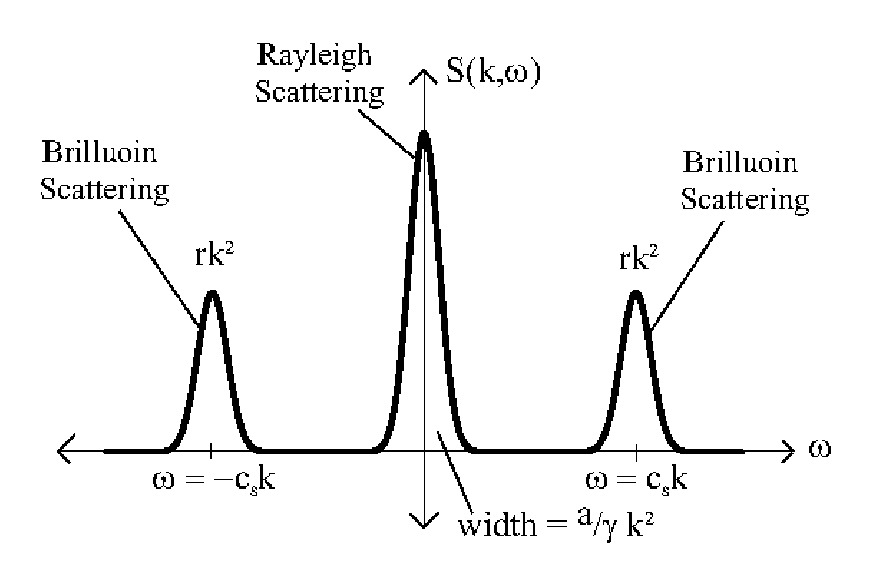
\[\hat{\rho}_{k}(t)=\hat{\rho_{k}}(0)\left[\left(1-\frac{1}{\gamma}\right) e^{-\frac{a}{\gamma} k^{2} t}+\frac{1}{\gamma} \cos \left(c_{S} k t\right) e^{-\Gamma k^{2} t}\right]\]

The first term gives the contributions from thermal fluctuations, while the second term gives the solution for a damped acoustic wave. Notice that the integrated intensity of the first term is \(\left(1-\frac{1}{\gamma}\right)\) and the integrated intensity of the second term is \(\frac{1}{\gamma}\).

Figure 3.9: Light Scattering Spectrum

Light Scattering

The Landau-Placzek ratio gives the ratio between the intensity of thermal and acoustic scattering

\[\frac{I_{\text {thermal }}}{I_{\text {acoustic }}}=\frac{\left\langle(\delta \rho)^{2}\right\rangle_{\text {thermal }}}{\left\langle(\delta \rho)^{2}\right\rangle_{\text {mech }}}=\frac{\left(\frac{\partial \rho}{\partial S}\right)_{P}^{2}\left\langle\Delta S^{2}\right\rangle}{\left(\frac{\partial \rho}{\partial P}\right)_{S}^{2}\left\langle\Delta P^{2}\right\rangle}=\frac{C_{P}-C_{V}}{C_{V}}=\gamma-1\]

Note that the dynamic structure factor is twice the real part of the Laplace transform of the intermediate scattering function (Figure 3.9):

\[S(\vec{k}, \omega)=\int_{\infty}^{\infty} F(\vec{k}, t) e^{-i \omega t} d t=2 \operatorname{Re} \hat{F}(z=-i \omega)\]

The initial value of this function is

\[F(k, 0)=\frac{1}{N}\left\langle\left|\delta \rho_{k}\right|^{2}\right\rangle=\rho_{o} h+1=\frac{\rho_{o} \chi_{T}}{\beta}\]

Acoustic Scattering

By ignoring the coupling to entropy flow, we have

\[d P=\left(\frac{\partial P}{\partial \rho}\right)_{S} d \rho\]

so that

\[\begin{array}{r} \frac{d \delta \rho_{k}}{d t}+i k \rho_{o} v_{k}=0 \\ \dot{v_{k}}+i c_{S}^{2} k \rho_{k}+b k^{2} v_{k}=0 \end{array}\]

For an ideal gas, \(b=0\), and so we get a propagating sound wave

\[z=\pm i c_{S} k\]

In a viscous liquid, \(b \neq 0\), and so we get a propagating acoustic wave with a damping term

\[z=\pm i c_{S} k-\frac{1}{2} b k^{2}\]