2.3: Linear Response Theory and Causality

The concept of linear response was introduced in section 2.1. Here, we explore further how the linear response of a system is quantified by considering the important relations regularly invoked by practitioners of linear response theory.

Response Functions

The motivating idea behind linear response is that the response of a system to an external force depends on the strength of that force at all times during which the force acts on the system. That is, the response at time \(t\) depends on the history of the force’s action on the system. An appropriately weighted sum of the strength of the external force at each moment during the interaction will describe the overall response. Mathematically, therefore, we express the response as an integral over the history of the interaction,

\[\Delta A(t)=\int_{-\infty}^{\infty} K(t, \tau) f(\tau) d \tau\]

The kernel \(K(t, \tau)\) in this expression, which provides the weight for the strength of the external force at each time, is called the response function. The response function has two very important properties:

• Time invariance: \(K\) depends only on the time interval between \(\tau\) and \(t\), not on the two times independently. More succinctly,

\[K(t, \tau)=K(t-\tau)\]

• Causality: The system cannot respond until the force has been applied. This places an upper limit of \(t\) on the integration over the history of the external force.

With these observations in place, we arrive at the standard formula describing the linear response of an observable \(A\) to an external force \(f(t)\),

\[\Delta A(t)=\int_{-\infty}^{t} K(t-\tau) f(\tau) d \tau\]

Linear response - described by the response function \(K(t)\) - and linear regression - described by the time correlation function \(C(t)\) - are directly related to one another. To see the connection, consider a force \(f(t)\) which is constant with strength \(f\) for \(t \leq 0\) and is zero for \(t>0\). We have established two ways to describe the response of an observable \(A\) to this force:

• Linear regression: \(\Delta A(t)=\beta f C(t)\)
• Linear response: \(\Delta A(t)=\int_{-\infty}^{0} K(t-\tau) f(\tau) d \tau\)

From this information, we conclude that the correlation function and response function are related by

\[K(t)=-\beta \dot{C}(t) \theta(t)\]

where \(\theta(t)\) is the Heaviside function.

Sometimes the linear response function is more conveniently expressed in the frequency domain, in which case it is called the frequency-dependent response function. In many physical situations, it plays the role of a susceptibility to a force and consequently is denoted by \(\chi(\omega)\),

\[\chi(\omega)=\int_{0}^{\infty} e^{i \omega t} K(t) d t\]

This response function is often partitioned into real and imaginary parts, which can also be thought of as even and odd parts, respectively,

\[\chi(\omega)=\chi^{\prime}(\omega)+i \chi^{\prime \prime}(\omega)\]

Example: The response function for the classical linear harmonic oscillator can be quickly deduced from its time correlation function. Recall from the first example in this chapter that the time correlation function for the classical linear harmonic oscillator is

\[C(t)=\frac{k_{B} T}{m \omega^{2}} \cos \omega t\]

Applying Eq.(2.17), we differentiate with respect to \(t\) and multiply by \(\beta=\frac{1}{k_{B} T}\) to determine that

\[K(t)=\frac{1}{m \omega} \sin (\omega t) \theta(t)\]

This is the response function for the classical linear harmonic oscillator.

Absorption Power Spectra

The frequency-dependent response function is directly related to the absorption spectrum: in fact, knowledge of \(\chi(\omega)\) and the time-dependent external force \(f(t)\) is sufficient to fully describe the absorption spectrum.

The rate at which work is done on a system by a generalized external force \(f(t)\) is \(f(t) \dot{A}(t)\), where \(A\) is the observable corresponding to the generalized force \(f\). This quantity has units of power, so we can calculate the total absorption energy by integrating this power over time,

\[\int P(t) d t=\int f(t) \dot{A}(t) d t\]

To recast this result in terms of \(\chi(\omega)\), we first consider the Fourier transform of the time-dependent observable \(A\),

\[\tilde{A}(\omega)=\int e^{i t} A(t) d t\]

Applying Eq.(2.16), we have

\[\tilde{A}(\omega)=\int e^{i \omega t} \int K(t-\tau) f(\tau) d \tau d t\]

The following rearrangements allow us to express \(\tilde{A}(\omega)\) entirely in terms of frequency-dependent functions:

\[\begin{aligned} \tilde{A}(\omega) &=\iint e^{i \omega(t-\tau)} e^{i \tau} K(t-\tau) f(\tau) d \tau d t \\ &=\int e^{i \omega(t-\tau)} K(t-\tau) d(t-\tau) \int e^{i \omega \tau} f(\tau) d t \\ &=\chi(\omega) \tilde{f}(\omega) \end{aligned}\]

where \(\tilde{f}(\omega)\) is the Fourier transform of \(f(t)\). Returning to Eq. (2.20) for the absorption energy,

\[\int P(t) d t=\int f(t) \dot{A}(t) d t=\frac{1}{2 \pi} \int \tilde{f}(-\omega) \tilde{\dot{A}}(\omega) d \omega\]

Rearranging the expression once again and evaluating the integral over time yields

\[\begin{aligned} \int P(t) d t &=\frac{1}{2 \pi} \int(-i \omega) \tilde{f}(-\omega) \tilde{A}(\omega) d \omega \\ &=\frac{1}{2 \pi} \int(-i \omega) \chi(\omega)|\tilde{f}(\omega)|^{2} d \omega \\ &=\frac{1}{2 \pi} \int \omega \chi^{\prime \prime}(\omega)|\tilde{f}(\omega)|^{2} d \omega \end{aligned}\]

Hence the absorption power spectrum \(P(\omega)\) has the form

\[P(\omega)=\omega \chi^{\prime \prime}(\omega)|\tilde{f}(\omega)|^{2}\]

Example: For a monochromatic force \(F(t)=F \cos \omega_{0} t\), the Fourier transform of \(F(t)\) is given by

\[\tilde{F}(\omega)=F \pi\left[\delta\left(\omega-\omega_{0}\right)+\delta\left(\omega+\omega_{0}\right)\right]\]

Hence our expression for the absorption power spectrum Eq.(2.30) tells us that the absorption rate (i.e. the time average of \(P(t)\) ) for such a system is

\[\lim _{\tau \rightarrow \infty} \frac{1}{\tau} \int_{0}^{\tau} P(t) d t=\frac{\omega}{2} \chi^{\prime \prime}(\omega)|F|^{2}\]

Furthermore, using Eq. \((2.17)\) and the fact that \(\chi^{\prime \prime}(\omega)\) is odd, we find that

\[\begin{aligned} \chi^{\prime \prime}(\omega) &=\int_{0}^{\infty} \sin \omega t K(t) d t \\ &=\int_{0}^{\infty} \sin \omega t(-\beta \dot{C}(t)) d t \\ &=\beta \omega \int_{0}^{\infty} C(t) \cos \omega t d t \\ &=\frac{\beta \omega}{2} \int_{-\infty}^{\infty} e^{i \omega t} C(t) d t \\ &=\frac{\beta \omega}{2} \tilde{C}(\omega) \end{aligned}\]

This simple relationship illustrates the close connection between frequency-dependent response functions (or susceptibilities) and time correlation functions.

Causality and the Kramers-Kronig Relations

Our final consideration in this chapter is the relationship between the real and imaginary parts of the frequency-dependent response function as defined in Eq.(2.19). The equations relating these two functions are known as the Kramers-Kronig relations. In their most general form, they govern the response function as a function of the complex frequency \(z=\omega+i \epsilon\), though under most physical circumstances of interest they can be expressed in terms of real-valued frequencies alone.

The relations arise from the causality requirement, which we originally expressed by requiring \(K(t)=0, \forall t<0\). It turns out that this requirement, along with the assumption that \(\int_{0}^{\infty} K(t) d t\) converges, implies that the response function \(\chi(z)\) is analytic on the upper half of the complex plane.

Figure 2.3: Contour in the complex frequency plane used to motivate the Kramers-Kronig relations

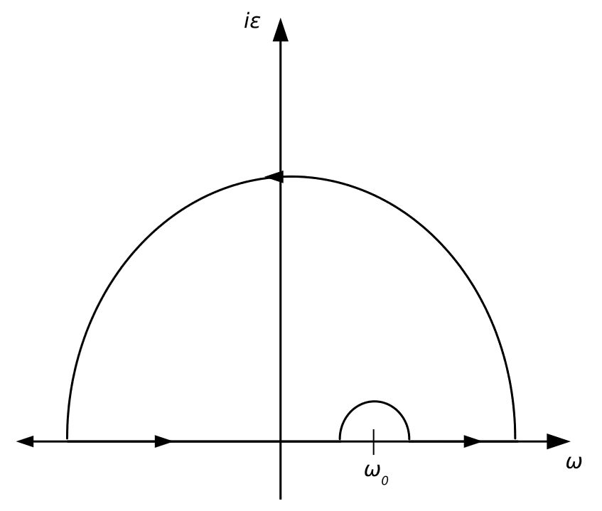
We can also, however, integrate piecewise over each part of the contour; some manipulation with the residue theorem is required, but the final result is

\[\oint \frac{\chi(z)}{z-\omega_{0}} d z=\mathcal{P} \int_{-\infty}^{\infty} \frac{\chi(z)}{z-\omega_{0}} d z-i \pi \chi\left(\omega_{0}\right)\]

where \(\mathcal{P}\) denotes the Cauchy principal value of the integral. Setting the two results above equal and solving for the response function,

\[\chi(\omega)=\frac{1}{i \pi} \mathcal{P} \int_{-\infty}^{\infty} \frac{\chi(z)}{z-\omega} d z\]

The decomposition of Eq.(2.33) into real and imaginary parts yields the Kramers-Kronig relations,

\[\begin{aligned} &\chi^{\prime}(\omega)=\frac{1}{\pi} \mathcal{P} \int_{-\infty}^{\infty} \frac{\chi^{\prime \prime}(z)}{z-\omega} d z \\ &\chi^{\prime \prime}(\omega)=-\frac{1}{\pi} \mathcal{P} \int_{-\infty}^{\infty} \frac{\chi^{\prime}(z)}{z-\omega} d z \end{aligned}\]

As promised, this pair of equations provides a concise relationship between the real and imaginary parts of any response function \(\chi(\omega)\).

References

[1] N. Kubo, R.; Saito and N. Hashitsume. Statistical Physics II: Nonequilibrium Statistical Mechanics. Springer, \(2003 .\)

[2] Robert Zwanzig. Nonequilibrium Statistical Mechanics. New York: Oxford University Press, \(2001 .\)

[3] David Chandler. Introduction to Modern Statistical Mechanics. New York: Oxford University Press, 1987 .

[4] L.E. Reichl. A Modern Course in Statistical Physics. New York: Wiley-Interscience, 1998 . MIT OpenCourseWare