12.4: Molecular Diffusion
- Page ID
- 106879

\( \newcommand{\vecs}[1]{\overset { \scriptstyle \rightharpoonup} {\mathbf{#1}} } \)
\( \newcommand{\vecd}[1]{\overset{-\!-\!\rightharpoonup}{\vphantom{a}\smash {#1}}} \)
\( \newcommand{\id}{\mathrm{id}}\) \( \newcommand{\Span}{\mathrm{span}}\)
( \newcommand{\kernel}{\mathrm{null}\,}\) \( \newcommand{\range}{\mathrm{range}\,}\)
\( \newcommand{\RealPart}{\mathrm{Re}}\) \( \newcommand{\ImaginaryPart}{\mathrm{Im}}\)
\( \newcommand{\Argument}{\mathrm{Arg}}\) \( \newcommand{\norm}[1]{\| #1 \|}\)
\( \newcommand{\inner}[2]{\langle #1, #2 \rangle}\)
\( \newcommand{\Span}{\mathrm{span}}\)
\( \newcommand{\id}{\mathrm{id}}\)
\( \newcommand{\Span}{\mathrm{span}}\)
\( \newcommand{\kernel}{\mathrm{null}\,}\)
\( \newcommand{\range}{\mathrm{range}\,}\)
\( \newcommand{\RealPart}{\mathrm{Re}}\)
\( \newcommand{\ImaginaryPart}{\mathrm{Im}}\)
\( \newcommand{\Argument}{\mathrm{Arg}}\)
\( \newcommand{\norm}[1]{\| #1 \|}\)
\( \newcommand{\inner}[2]{\langle #1, #2 \rangle}\)
\( \newcommand{\Span}{\mathrm{span}}\) \( \newcommand{\AA}{\unicode[.8,0]{x212B}}\)
\( \newcommand{\vectorA}[1]{\vec{#1}} % arrow\)
\( \newcommand{\vectorAt}[1]{\vec{\text{#1}}} % arrow\)
\( \newcommand{\vectorB}[1]{\overset { \scriptstyle \rightharpoonup} {\mathbf{#1}} } \)
\( \newcommand{\vectorC}[1]{\textbf{#1}} \)
\( \newcommand{\vectorD}[1]{\overrightarrow{#1}} \)
\( \newcommand{\vectorDt}[1]{\overrightarrow{\text{#1}}} \)
\( \newcommand{\vectE}[1]{\overset{-\!-\!\rightharpoonup}{\vphantom{a}\smash{\mathbf {#1}}}} \)
\( \newcommand{\vecs}[1]{\overset { \scriptstyle \rightharpoonup} {\mathbf{#1}} } \)
\( \newcommand{\vecd}[1]{\overset{-\!-\!\rightharpoonup}{\vphantom{a}\smash {#1}}} \)
\(\newcommand{\avec}{\mathbf a}\) \(\newcommand{\bvec}{\mathbf b}\) \(\newcommand{\cvec}{\mathbf c}\) \(\newcommand{\dvec}{\mathbf d}\) \(\newcommand{\dtil}{\widetilde{\mathbf d}}\) \(\newcommand{\evec}{\mathbf e}\) \(\newcommand{\fvec}{\mathbf f}\) \(\newcommand{\nvec}{\mathbf n}\) \(\newcommand{\pvec}{\mathbf p}\) \(\newcommand{\qvec}{\mathbf q}\) \(\newcommand{\svec}{\mathbf s}\) \(\newcommand{\tvec}{\mathbf t}\) \(\newcommand{\uvec}{\mathbf u}\) \(\newcommand{\vvec}{\mathbf v}\) \(\newcommand{\wvec}{\mathbf w}\) \(\newcommand{\xvec}{\mathbf x}\) \(\newcommand{\yvec}{\mathbf y}\) \(\newcommand{\zvec}{\mathbf z}\) \(\newcommand{\rvec}{\mathbf r}\) \(\newcommand{\mvec}{\mathbf m}\) \(\newcommand{\zerovec}{\mathbf 0}\) \(\newcommand{\onevec}{\mathbf 1}\) \(\newcommand{\real}{\mathbb R}\) \(\newcommand{\twovec}[2]{\left[\begin{array}{r}#1 \\ #2 \end{array}\right]}\) \(\newcommand{\ctwovec}[2]{\left[\begin{array}{c}#1 \\ #2 \end{array}\right]}\) \(\newcommand{\threevec}[3]{\left[\begin{array}{r}#1 \\ #2 \\ #3 \end{array}\right]}\) \(\newcommand{\cthreevec}[3]{\left[\begin{array}{c}#1 \\ #2 \\ #3 \end{array}\right]}\) \(\newcommand{\fourvec}[4]{\left[\begin{array}{r}#1 \\ #2 \\ #3 \\ #4 \end{array}\right]}\) \(\newcommand{\cfourvec}[4]{\left[\begin{array}{c}#1 \\ #2 \\ #3 \\ #4 \end{array}\right]}\) \(\newcommand{\fivevec}[5]{\left[\begin{array}{r}#1 \\ #2 \\ #3 \\ #4 \\ #5 \\ \end{array}\right]}\) \(\newcommand{\cfivevec}[5]{\left[\begin{array}{c}#1 \\ #2 \\ #3 \\ #4 \\ #5 \\ \end{array}\right]}\) \(\newcommand{\mattwo}[4]{\left[\begin{array}{rr}#1 \amp #2 \\ #3 \amp #4 \\ \end{array}\right]}\) \(\newcommand{\laspan}[1]{\text{Span}\{#1\}}\) \(\newcommand{\bcal}{\cal B}\) \(\newcommand{\ccal}{\cal C}\) \(\newcommand{\scal}{\cal S}\) \(\newcommand{\wcal}{\cal W}\) \(\newcommand{\ecal}{\cal E}\) \(\newcommand{\coords}[2]{\left\{#1\right\}_{#2}}\) \(\newcommand{\gray}[1]{\color{gray}{#1}}\) \(\newcommand{\lgray}[1]{\color{lightgray}{#1}}\) \(\newcommand{\rank}{\operatorname{rank}}\) \(\newcommand{\row}{\text{Row}}\) \(\newcommand{\col}{\text{Col}}\) \(\renewcommand{\row}{\text{Row}}\) \(\newcommand{\nul}{\text{Nul}}\) \(\newcommand{\var}{\text{Var}}\) \(\newcommand{\corr}{\text{corr}}\) \(\newcommand{\len}[1]{\left|#1\right|}\) \(\newcommand{\bbar}{\overline{\bvec}}\) \(\newcommand{\bhat}{\widehat{\bvec}}\) \(\newcommand{\bperp}{\bvec^\perp}\) \(\newcommand{\xhat}{\widehat{\xvec}}\) \(\newcommand{\vhat}{\widehat{\vvec}}\) \(\newcommand{\uhat}{\widehat{\uvec}}\) \(\newcommand{\what}{\widehat{\wvec}}\) \(\newcommand{\Sighat}{\widehat{\Sigma}}\) \(\newcommand{\lt}{<}\) \(\newcommand{\gt}{>}\) \(\newcommand{\amp}{&}\) \(\definecolor{fillinmathshade}{gray}{0.9}\)Molecular diffusion is the thermal motion of molecules at temperatures above absolute zero. The rate of this movement is a function of temperature, viscosity of the fluid and the size and shape of the particles. Diffusion explains the net flux of molecules from a region of higher concentration to one of lower concentration. The term "diffusion" is also generally used to describe the flux of other physical quantities. For instance, the diffusion of thermal energy (heat) is described by the heat equation, which is mathematically identical to the diffusion equation we’ll consider in this section.
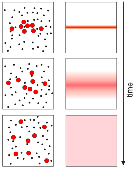
To visualize what we mean by molecular diffusion, consider a red dye diffusing in a test tube. Suppose the experiment starts by placing a sample of the dye in a thin layer half way down the tube. Diffusion occurs because all molecules move due to their thermal energy. Each molecule moves in a random direction, meaning that if you wait long enough, molecules will end up being randomly distributed throughout the tube. This means that there is a net movement of dye molecules from areas of high concentration (the central band) into areas of low concentration (Figure \(\PageIndex{1}\). The rate of diffusion depends on temperature, the size and shape of the molecules, and the viscosity of the solvent.
The diffusion equation that describes how the concentration of solute (in this case the red dye) changes with position and time is:
\[\label{eq:pde31} \nabla^2C(\mathbf{r},t)=\frac{1}{D}\frac{\partial C(\mathbf{r},t)}{\partial t} \]
where \(\mathbf{r}\) is a vector representing the position in a particular coordinate system. This equation is known as Fick’s second law of diffusion, and its solution depends on the dimensionality of the problem (1D, 2D, 3D), and the initial and boundary conditions. If molecules are able to move in one dimension only (for example in a tube that is much longer than its diameter):
\[\label{eq:pde32} \frac{\partial^2C(x,t)}{\partial x^2}=\frac{1}{D}\frac{\partial C(x,t)}{\partial t} \]
Let’s assume that the tube has a length \(L\) and it is closed at both ends. Mathematically, this means that the flux of molecules at \(x = 0\) and \(x = L\) is zero. The flux is defined as the number of moles of substance that cross a \(1 m^2\) area per second, and it is mathematically defined as
\[\label{eq:pde33} J=-D\frac{\partial C(x,t)}{\partial x} \]
If the tube is closed, molecules at \(x=0\) cannot move from the right side to the left side, and molecules at \(x=L\) cannot move from the left side to the right side. Mathematically:
\[\label{eq:pde34} \frac{\partial C(0,t)}{\partial x}=\frac{\partial C(L,t)}{\partial x}=0 \]
These will be the boundary conditions we will use to solve the problem We still need an initial condition, which in this case it is the initial concentration profile: \(C(x,0)=y(x)\). Notice that because of mass conservation, the integral of \(C(x)\) should be constant at all times. We will not use this to solve the problem, but we can verify that the solution satisfies this requirement.
Regardless of initial conditions, the concentration profile will be expressed as (Problem 12.3):
\[\label{eq:pde_35} C(x,t)=\sum\limits_{n=0}^{\infty}a_n\cos\left(\frac{n\pi}{L}x \right)e^{-\left(\frac{n\pi}{L}\right)^2Dt} \]
In order to calculate the coefficients \(a_n\), we need information about the initial concentration profile: \(C(x,0)=y(x)\).
\[\label{eq:pde_36} C(x,0)=\sum\limits_{n=0}^{\infty}a_n\cos\left(\frac{n\pi}{L}x \right)=y(x) \]
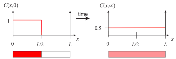
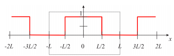
This expression tells us that the function \(y(x)\) can be expressed as an infinite sum of cosines. We know from Chapter 7 that an infinite sum of cosines like this represents an even periodic function of period \(2L\), so in order to find the coefficients \(a_n\), we need to construct the even periodic extension of the function \(y(x)\) and find its Fourier series. For example, assume that the initial concentration profile is given by Figure \(\PageIndex{2}\). Imagine that you have water in the right half-side of the tube, and a 1M solution of red dye on the left half-side. At time zero, you remove the barrier that separates the two halves, and watch the concentration evolve as a function of time. Before we calculate these concentration profiles, let’s think about what we expect at very long times, when the dye is allowed to fully mix with the water. We know that the same number of molecules present initially need to be re-distributed in the full length of the tube, so the concentration profile needs to be constant at 0.5M. It is a good idea that you sketch what you imagine happens in between before going through the math and seeing the results.
In order to calculate the coefficients \(a_n\) that we need to complete Equation \ref{eq:pde_35}, we need to express \(C(x,0)\) as an infinite sum of cosine functions, and therefore we need the even extension of the function:
Let’s calculate the Fourier series of this periodic function of period \(2L\) (Equation \(7.2.1\), \( f(x)=\dfrac{a_0}{2}+\sum_{n=1}^{\infty}a_n \cos\left ( \dfrac{n\pi x}{L} \right )+\sum_{n=1}^{\infty}b_n \sin\left ( \dfrac{n\pi x}{L} \right )\) ).
\[f(x)=\frac{a_0}{2}+\sum_{n=1}^{\infty}a_n cos\left ( \frac{n\pi x}{L} \right ) \nonumber \]
\[a_0=\frac{1}{L}\int_{-L}^{L}f(x)dx \nonumber \]
\[a_n=\frac{1}{L}\int_{-L}^{L}f(x)\cos{\left(\frac{n\pi x}{L} \right)}dx \nonumber \]
Let’s assume \(L=1cm\) (we will use \(D\) in units of \(cm^2/s\) and \(t\) in seconds):
\[a_0=\frac{1}{L}\int_{-L}^{L}f(x)dx=\int_{-1/2}^{1/2}1dx=1 \nonumber \]
\[a_n=\int_{-1/2}^{1/2}1\cos{\left(n\pi x\right)}dx=\frac{1}{n\pi}\left.\begin{matrix}\sin(n\pi x)\end{matrix}\right|_{-1/2}^{1/2}=\frac{1}{n\pi}[\sin{(n\pi/2)}-\sin{(-n\pi/2)}] \nonumber \]
because \(\sin{x}\) is odd:
\[a_n=\frac{2}{n\pi}\sin{(n\pi/2)}\rightarrow a_1=\frac{2}{\pi}, a_2=0, a_3=-\frac{2}{3\pi}, a_4=0, a_5=\frac{2}{5\pi}... \nonumber \]
and therefore:
\[C(x,0)=\frac{1}{2}+\frac{2}{\pi}\sum\limits_{n=0}^{\infty}(-1)^{n}\frac{1}{2n+1}\cos{[(2n+1)\pi x]} \nonumber \]
and the complete description of \(C(x,t)\) is (Equation \ref{eq:pde_35}):
\[\label{eq:pde_37} C(x,t)=\frac{1}{2}+\frac{2}{\pi}\sum\limits_{n=0}^{\infty}(-1)^{n}\frac{1}{2n+1}\cos{[(2n+1)\pi x]}e^{-[(2n+1)\pi]^2Dt} \]
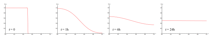
Let’s plot \(C(x,t)\) at different times assuming \(L=1cm\) and \(D=6.5 \times 10^{-6}cm^2 s^{-1}\), which is the diffusion coefficient of sucrose (regular sugar) in water.
Notice that the derivative \(\frac{\partial C(x,t)}{\partial x}\) is zero at both \(x=0\) and \(x=L=1cm\) at all times, as it should be the case given the boundary conditions. Also, the area under the curve is constant due to mass conservation. In addition notice how long it takes for diffusion to mix the two halves of the tube! It would take about a day for the concentration to be relatively homogeneous in a 1-cm tube, which explains why it is a good idea to stir the sugar in your coffee with a spoon instead of waiting for diffusion to do the job. Diffusion is inefficient because molecules move in random directions, and each time they bump into a molecule of water they change their direction. Imagine that you need to walk from the corner of Apache and Rural to the corner of College and University Ave, and every time you make a step you throw a four-sided die to decide whether to move south, north, east or west. You might eventually get to your destination, but it will likely take you a long time.