10.1: Coordinate Systems
- Page ID
- 106862

\( \newcommand{\vecs}[1]{\overset { \scriptstyle \rightharpoonup} {\mathbf{#1}} } \)
\( \newcommand{\vecd}[1]{\overset{-\!-\!\rightharpoonup}{\vphantom{a}\smash {#1}}} \)
\( \newcommand{\id}{\mathrm{id}}\) \( \newcommand{\Span}{\mathrm{span}}\)
( \newcommand{\kernel}{\mathrm{null}\,}\) \( \newcommand{\range}{\mathrm{range}\,}\)
\( \newcommand{\RealPart}{\mathrm{Re}}\) \( \newcommand{\ImaginaryPart}{\mathrm{Im}}\)
\( \newcommand{\Argument}{\mathrm{Arg}}\) \( \newcommand{\norm}[1]{\| #1 \|}\)
\( \newcommand{\inner}[2]{\langle #1, #2 \rangle}\)
\( \newcommand{\Span}{\mathrm{span}}\)
\( \newcommand{\id}{\mathrm{id}}\)
\( \newcommand{\Span}{\mathrm{span}}\)
\( \newcommand{\kernel}{\mathrm{null}\,}\)
\( \newcommand{\range}{\mathrm{range}\,}\)
\( \newcommand{\RealPart}{\mathrm{Re}}\)
\( \newcommand{\ImaginaryPart}{\mathrm{Im}}\)
\( \newcommand{\Argument}{\mathrm{Arg}}\)
\( \newcommand{\norm}[1]{\| #1 \|}\)
\( \newcommand{\inner}[2]{\langle #1, #2 \rangle}\)
\( \newcommand{\Span}{\mathrm{span}}\) \( \newcommand{\AA}{\unicode[.8,0]{x212B}}\)
\( \newcommand{\vectorA}[1]{\vec{#1}} % arrow\)
\( \newcommand{\vectorAt}[1]{\vec{\text{#1}}} % arrow\)
\( \newcommand{\vectorB}[1]{\overset { \scriptstyle \rightharpoonup} {\mathbf{#1}} } \)
\( \newcommand{\vectorC}[1]{\textbf{#1}} \)
\( \newcommand{\vectorD}[1]{\overrightarrow{#1}} \)
\( \newcommand{\vectorDt}[1]{\overrightarrow{\text{#1}}} \)
\( \newcommand{\vectE}[1]{\overset{-\!-\!\rightharpoonup}{\vphantom{a}\smash{\mathbf {#1}}}} \)
\( \newcommand{\vecs}[1]{\overset { \scriptstyle \rightharpoonup} {\mathbf{#1}} } \)
\( \newcommand{\vecd}[1]{\overset{-\!-\!\rightharpoonup}{\vphantom{a}\smash {#1}}} \)
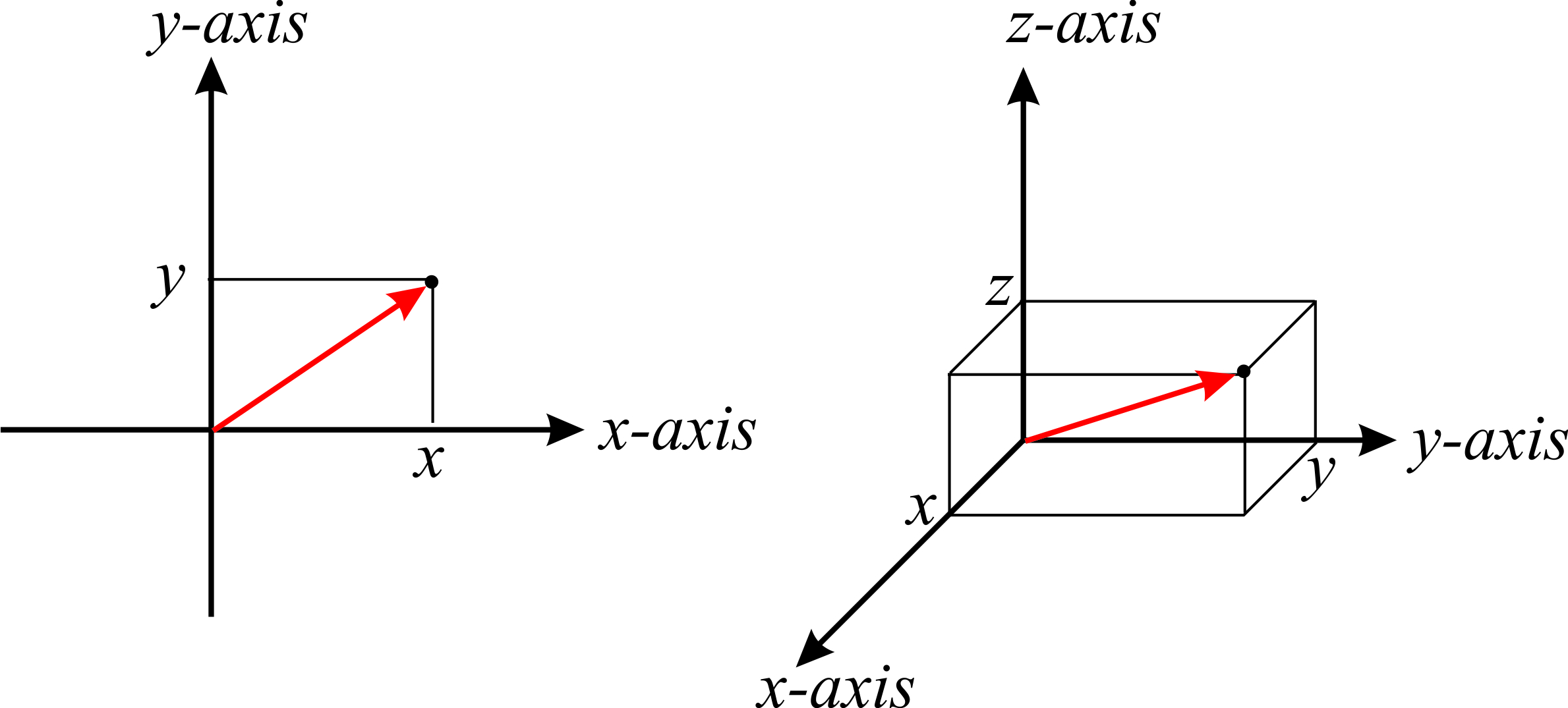
\(\newcommand{\avec}{\mathbf a}\) \(\newcommand{\bvec}{\mathbf b}\) \(\newcommand{\cvec}{\mathbf c}\) \(\newcommand{\dvec}{\mathbf d}\) \(\newcommand{\dtil}{\widetilde{\mathbf d}}\) \(\newcommand{\evec}{\mathbf e}\) \(\newcommand{\fvec}{\mathbf f}\) \(\newcommand{\nvec}{\mathbf n}\) \(\newcommand{\pvec}{\mathbf p}\) \(\newcommand{\qvec}{\mathbf q}\) \(\newcommand{\svec}{\mathbf s}\) \(\newcommand{\tvec}{\mathbf t}\) \(\newcommand{\uvec}{\mathbf u}\) \(\newcommand{\vvec}{\mathbf v}\) \(\newcommand{\wvec}{\mathbf w}\) \(\newcommand{\xvec}{\mathbf x}\) \(\newcommand{\yvec}{\mathbf y}\) \(\newcommand{\zvec}{\mathbf z}\) \(\newcommand{\rvec}{\mathbf r}\) \(\newcommand{\mvec}{\mathbf m}\) \(\newcommand{\zerovec}{\mathbf 0}\) \(\newcommand{\onevec}{\mathbf 1}\) \(\newcommand{\real}{\mathbb R}\) \(\newcommand{\twovec}[2]{\left[\begin{array}{r}#1 \\ #2 \end{array}\right]}\) \(\newcommand{\ctwovec}[2]{\left[\begin{array}{c}#1 \\ #2 \end{array}\right]}\) \(\newcommand{\threevec}[3]{\left[\begin{array}{r}#1 \\ #2 \\ #3 \end{array}\right]}\) \(\newcommand{\cthreevec}[3]{\left[\begin{array}{c}#1 \\ #2 \\ #3 \end{array}\right]}\) \(\newcommand{\fourvec}[4]{\left[\begin{array}{r}#1 \\ #2 \\ #3 \\ #4 \end{array}\right]}\) \(\newcommand{\cfourvec}[4]{\left[\begin{array}{c}#1 \\ #2 \\ #3 \\ #4 \end{array}\right]}\) \(\newcommand{\fivevec}[5]{\left[\begin{array}{r}#1 \\ #2 \\ #3 \\ #4 \\ #5 \\ \end{array}\right]}\) \(\newcommand{\cfivevec}[5]{\left[\begin{array}{c}#1 \\ #2 \\ #3 \\ #4 \\ #5 \\ \end{array}\right]}\) \(\newcommand{\mattwo}[4]{\left[\begin{array}{rr}#1 \amp #2 \\ #3 \amp #4 \\ \end{array}\right]}\) \(\newcommand{\laspan}[1]{\text{Span}\{#1\}}\) \(\newcommand{\bcal}{\cal B}\) \(\newcommand{\ccal}{\cal C}\) \(\newcommand{\scal}{\cal S}\) \(\newcommand{\wcal}{\cal W}\) \(\newcommand{\ecal}{\cal E}\) \(\newcommand{\coords}[2]{\left\{#1\right\}_{#2}}\) \(\newcommand{\gray}[1]{\color{gray}{#1}}\) \(\newcommand{\lgray}[1]{\color{lightgray}{#1}}\) \(\newcommand{\rank}{\operatorname{rank}}\) \(\newcommand{\row}{\text{Row}}\) \(\newcommand{\col}{\text{Col}}\) \(\renewcommand{\row}{\text{Row}}\) \(\newcommand{\nul}{\text{Nul}}\) \(\newcommand{\var}{\text{Var}}\) \(\newcommand{\corr}{\text{corr}}\) \(\newcommand{\len}[1]{\left|#1\right|}\) \(\newcommand{\bbar}{\overline{\bvec}}\) \(\newcommand{\bhat}{\widehat{\bvec}}\) \(\newcommand{\bperp}{\bvec^\perp}\) \(\newcommand{\xhat}{\widehat{\xvec}}\) \(\newcommand{\vhat}{\widehat{\vvec}}\) \(\newcommand{\uhat}{\widehat{\uvec}}\) \(\newcommand{\what}{\widehat{\wvec}}\) \(\newcommand{\Sighat}{\widehat{\Sigma}}\) \(\newcommand{\lt}{<}\) \(\newcommand{\gt}{>}\) \(\newcommand{\amp}{&}\) \(\definecolor{fillinmathshade}{gray}{0.9}\)The simplest coordinate system consists of coordinate axes oriented perpendicularly to each other. These coordinates are known as cartesian coordinates or rectangular coordinates, and you are already familiar with their two-dimensional and three-dimensional representation. In the plane, any point \(P\) can be represented by two signed numbers, usually written as \((x,y)\), where the coordinate \(x\) is the distance perpendicular to the \(x\) axis, and the coordinate \(y\) is the distance perpendicular to the \(y\) axis (Figure \(\PageIndex{1}\), left). In space, a point is represented by three signed numbers, usually written as \((x,y,z)\) (Figure \(\PageIndex{1}\), right).
Often, positions are represented by a vector, \(\vec{r}\), shown in red in Figure \(\PageIndex{1}\). In three dimensions, this vector can be expressed in terms of the coordinate values as \(\vec{r}=x\hat{i}+y\hat{j}+z\hat{k}\), where \(\hat{i}=(1,0,0)\), \(\hat{j}=(0,1,0)\) and \(\hat{z}=(0,0,1)\) are the so-called unit vectors.
We already know that often the symmetry of a problem makes it natural (and easier!) to use other coordinate systems. In two dimensions, the polar coordinate system defines a point in the plane by two numbers: the distance \(r\) to the origin, and the angle \(\theta\) that the position vector forms with the \(x\)-axis. Notice the difference between \(\vec{r}\), a vector, and \(r\), the distance to the origin (and therefore the modulus of the vector). Vectors are often denoted in bold face (e.g. r) without the arrow on top, so be careful not to confuse it with \(r\), which is a scalar.
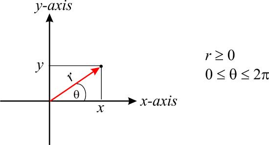
While in cartesian coordinates \(x\), \(y\) (and \(z\) in three-dimensions) can take values from \(-\infty\) to \(\infty\), in polar coordinates \(r\) is a positive value (consistent with a distance), and \(\theta\) can take values in the range \([0,2\pi]\).
The relationship between the cartesian and polar coordinates in two dimensions can be summarized as:
\[\label{eq:coordinates_1} x=r\cos\theta \]
\[\label{eq:coordinates_2} y=r\sin\theta \]
\[\label{eq:coordinates_3} r^2=x^2+y^2 \]
\[\label{eq:coordinates_4} \tan \theta=y/x \]
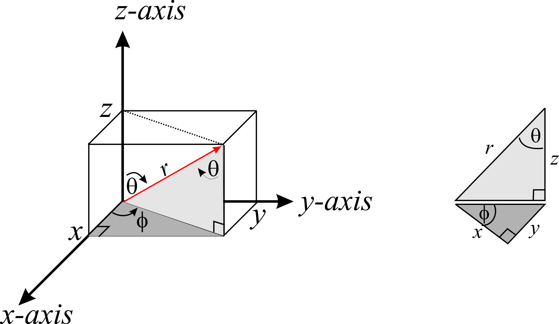
In three dimensions, the spherical coordinate system defines a point in space by three numbers: the distance \(r\) to the origin, a polar angle \(\phi\) that measures the angle between the positive \(x\)-axis and the line from the origin to the point \(P\) projected onto the \(xy\)-plane, and the angle \(\theta\) defined as the is the angle between the \(z\)-axis and the line from the origin to the point \(P\):
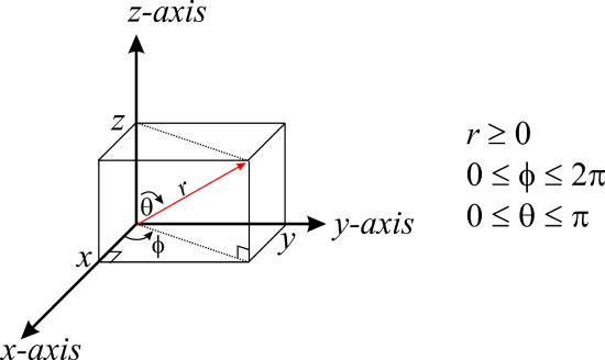
Before we move on, it is important to mention that depending on the field, you may see the Greek letter \(\theta\) (instead of \(\phi\)) used for the angle between the positive \(x\)-axis and the line from the origin to the point \(P\) projected onto the \(xy\)-plane. That is, \(\theta\) and \(\phi\) may appear interchanged. This can be very confusing, so you will have to be careful. When using spherical coordinates, it is important that you see how these two angles are defined so you can identify which is which.
Spherical coordinates are useful in analyzing systems that are symmetrical about a point. For example a sphere that has the cartesian equation \(x^2+y^2+z^2=R^2\) has the very simple equation \(r = R\) in spherical coordinates. Spherical coordinates are the natural coordinates for physical situations where there is spherical symmetry (e.g. atoms). The relationship between the cartesian coordinates and the spherical coordinates can be summarized as:
\[\label{eq:coordinates_5} x=r\sin\theta\cos\phi \]
\[\label{eq:coordinates_6} y=r\sin\theta\sin\phi \]
\[\label{eq:coordinates_7} z=r\cos\theta \]
These relationships are not hard to derive if one considers the triangles shown in Figure \(\PageIndex{4}\):