2.2: Graphical Representation and Euler Relationship
- Page ID
- 106807
\( \newcommand{\vecs}[1]{\overset { \scriptstyle \rightharpoonup} {\mathbf{#1}} } \)
\( \newcommand{\vecd}[1]{\overset{-\!-\!\rightharpoonup}{\vphantom{a}\smash {#1}}} \)
\( \newcommand{\id}{\mathrm{id}}\) \( \newcommand{\Span}{\mathrm{span}}\)
( \newcommand{\kernel}{\mathrm{null}\,}\) \( \newcommand{\range}{\mathrm{range}\,}\)
\( \newcommand{\RealPart}{\mathrm{Re}}\) \( \newcommand{\ImaginaryPart}{\mathrm{Im}}\)
\( \newcommand{\Argument}{\mathrm{Arg}}\) \( \newcommand{\norm}[1]{\| #1 \|}\)
\( \newcommand{\inner}[2]{\langle #1, #2 \rangle}\)
\( \newcommand{\Span}{\mathrm{span}}\)
\( \newcommand{\id}{\mathrm{id}}\)
\( \newcommand{\Span}{\mathrm{span}}\)
\( \newcommand{\kernel}{\mathrm{null}\,}\)
\( \newcommand{\range}{\mathrm{range}\,}\)
\( \newcommand{\RealPart}{\mathrm{Re}}\)
\( \newcommand{\ImaginaryPart}{\mathrm{Im}}\)
\( \newcommand{\Argument}{\mathrm{Arg}}\)
\( \newcommand{\norm}[1]{\| #1 \|}\)
\( \newcommand{\inner}[2]{\langle #1, #2 \rangle}\)
\( \newcommand{\Span}{\mathrm{span}}\) \( \newcommand{\AA}{\unicode[.8,0]{x212B}}\)
\( \newcommand{\vectorA}[1]{\vec{#1}} % arrow\)
\( \newcommand{\vectorAt}[1]{\vec{\text{#1}}} % arrow\)
\( \newcommand{\vectorB}[1]{\overset { \scriptstyle \rightharpoonup} {\mathbf{#1}} } \)
\( \newcommand{\vectorC}[1]{\textbf{#1}} \)
\( \newcommand{\vectorD}[1]{\overrightarrow{#1}} \)
\( \newcommand{\vectorDt}[1]{\overrightarrow{\text{#1}}} \)
\( \newcommand{\vectE}[1]{\overset{-\!-\!\rightharpoonup}{\vphantom{a}\smash{\mathbf {#1}}}} \)
\( \newcommand{\vecs}[1]{\overset { \scriptstyle \rightharpoonup} {\mathbf{#1}} } \)
\( \newcommand{\vecd}[1]{\overset{-\!-\!\rightharpoonup}{\vphantom{a}\smash {#1}}} \)
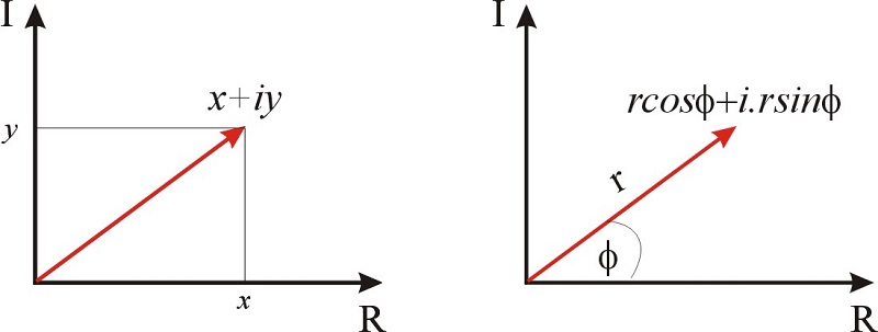
\(\newcommand{\avec}{\mathbf a}\) \(\newcommand{\bvec}{\mathbf b}\) \(\newcommand{\cvec}{\mathbf c}\) \(\newcommand{\dvec}{\mathbf d}\) \(\newcommand{\dtil}{\widetilde{\mathbf d}}\) \(\newcommand{\evec}{\mathbf e}\) \(\newcommand{\fvec}{\mathbf f}\) \(\newcommand{\nvec}{\mathbf n}\) \(\newcommand{\pvec}{\mathbf p}\) \(\newcommand{\qvec}{\mathbf q}\) \(\newcommand{\svec}{\mathbf s}\) \(\newcommand{\tvec}{\mathbf t}\) \(\newcommand{\uvec}{\mathbf u}\) \(\newcommand{\vvec}{\mathbf v}\) \(\newcommand{\wvec}{\mathbf w}\) \(\newcommand{\xvec}{\mathbf x}\) \(\newcommand{\yvec}{\mathbf y}\) \(\newcommand{\zvec}{\mathbf z}\) \(\newcommand{\rvec}{\mathbf r}\) \(\newcommand{\mvec}{\mathbf m}\) \(\newcommand{\zerovec}{\mathbf 0}\) \(\newcommand{\onevec}{\mathbf 1}\) \(\newcommand{\real}{\mathbb R}\) \(\newcommand{\twovec}[2]{\left[\begin{array}{r}#1 \\ #2 \end{array}\right]}\) \(\newcommand{\ctwovec}[2]{\left[\begin{array}{c}#1 \\ #2 \end{array}\right]}\) \(\newcommand{\threevec}[3]{\left[\begin{array}{r}#1 \\ #2 \\ #3 \end{array}\right]}\) \(\newcommand{\cthreevec}[3]{\left[\begin{array}{c}#1 \\ #2 \\ #3 \end{array}\right]}\) \(\newcommand{\fourvec}[4]{\left[\begin{array}{r}#1 \\ #2 \\ #3 \\ #4 \end{array}\right]}\) \(\newcommand{\cfourvec}[4]{\left[\begin{array}{c}#1 \\ #2 \\ #3 \\ #4 \end{array}\right]}\) \(\newcommand{\fivevec}[5]{\left[\begin{array}{r}#1 \\ #2 \\ #3 \\ #4 \\ #5 \\ \end{array}\right]}\) \(\newcommand{\cfivevec}[5]{\left[\begin{array}{c}#1 \\ #2 \\ #3 \\ #4 \\ #5 \\ \end{array}\right]}\) \(\newcommand{\mattwo}[4]{\left[\begin{array}{rr}#1 \amp #2 \\ #3 \amp #4 \\ \end{array}\right]}\) \(\newcommand{\laspan}[1]{\text{Span}\{#1\}}\) \(\newcommand{\bcal}{\cal B}\) \(\newcommand{\ccal}{\cal C}\) \(\newcommand{\scal}{\cal S}\) \(\newcommand{\wcal}{\cal W}\) \(\newcommand{\ecal}{\cal E}\) \(\newcommand{\coords}[2]{\left\{#1\right\}_{#2}}\) \(\newcommand{\gray}[1]{\color{gray}{#1}}\) \(\newcommand{\lgray}[1]{\color{lightgray}{#1}}\) \(\newcommand{\rank}{\operatorname{rank}}\) \(\newcommand{\row}{\text{Row}}\) \(\newcommand{\col}{\text{Col}}\) \(\renewcommand{\row}{\text{Row}}\) \(\newcommand{\nul}{\text{Nul}}\) \(\newcommand{\var}{\text{Var}}\) \(\newcommand{\corr}{\text{corr}}\) \(\newcommand{\len}[1]{\left|#1\right|}\) \(\newcommand{\bbar}{\overline{\bvec}}\) \(\newcommand{\bhat}{\widehat{\bvec}}\) \(\newcommand{\bperp}{\bvec^\perp}\) \(\newcommand{\xhat}{\widehat{\xvec}}\) \(\newcommand{\vhat}{\widehat{\vvec}}\) \(\newcommand{\uhat}{\widehat{\uvec}}\) \(\newcommand{\what}{\widehat{\wvec}}\) \(\newcommand{\Sighat}{\widehat{\Sigma}}\) \(\newcommand{\lt}{<}\) \(\newcommand{\gt}{>}\) \(\newcommand{\amp}{&}\) \(\definecolor{fillinmathshade}{gray}{0.9}\)Complex numbers can be represented graphically as a point in a coordinate plane. In cartesian coordinates, the \(x\)-axis is used for the real part of the number, and the \(y\)-axis is used for the imaginary component. For example, the complex number \(x+iy\) is represented as a point in Figure \(\PageIndex{1}\).
Complex numbers can be also represented in polar form. We know that, given a point \((x,y)\) in the plane, \(\cos\phi=x/r\) and \(\sin\phi=y/r\). Therefore, the complex number \(x+iy\) can be also represented as \(r\cos\phi+i r\sin\phi\).

We can also represent complex numbers in terms of complex exponentials. This will sound weird for now, but we will see how common and useful this is in physical chemistry as we cover other topics this semester. The Euler relationship relates the trigonometric functions to a complex exponential:
\[\label{eq1} e^{\pm i\phi}=\cos\phi\pm i\sin\phi \]
We will prove this relationship using Taylor series later.
In summary, the complex number \(\displaystyle{\color{Maroon} x+iy}\) can be expressed in polar coordinates as \(\displaystyle{\color{Maroon}r\cos\phi+i r\sin\phi}\), and as a complex exponential as \(\displaystyle{\color{Maroon}r e^{i\phi}}\). The relationships between \(x,y\) and \(r,\phi\) are given by the familiar trigonometric relationships: \(x=r\cos\phi\) and \(y=r\sin\phi\). Notice that
\[r^2=x^2+y^2 \nonumber \]
and
\[\sin^2\phi+\cos^2\phi=1 \nonumber \]
as we know from Pythagoras’ theorem.
Express \(z= 1+i\) in the form \(r e^{i\phi}\)
Solution
\(x = 1\) and \(y=1\).
We know that
\(x=r\cos\phi\) and \(y=r\sin\phi\)
Dividing \(y/x\), we get \(y/x=\tan\phi\). In this problem \(y=x\), and therefore \(\pi/4\).
To obtain \(r\) we use \(r^2=x^2+y^2\). In this case:
\[x^2+y^2=2 \to r=\sqrt{2} \nonumber \]
Therefore, \(\displaystyle{\color{Maroon}z = \sqrt{2} e^{\frac{\pi}{4} i}}\)
From Equation \ref{eq1} we can see how the trigonometric functions can be expressed as complex exponentials:
\[ \begin{split} \cos\phi=\frac{e^{i \phi}+e^{-i \phi}}{2}\\ \sin\phi=\frac{e^{i \phi}-e^{-i \phi}}{2i} \end{split} \nonumber \]
Again, this may look strange at this point, but it turns out that exponentials are much easier to manipulate than trigonometric functions (think about multiplying or dividing exponentials vs. trigonometric functions), so it is common that physical chemists write equations in terms of complex exponentials instead of cosines and sines.
In Equation \(2.1.1\) we saw that \((x+iy)(x-iy)=x^2+y^2\). Now we know that this equals \(r^2\), where \(r\) is the modulus or absolute value of the vector represented in red in Figure \(\PageIndex{1}\). Therefore, the modulus of a complex number, denoted as \(|z|\), can be calculated as:
\[\label{modulus} |z|^2= z z^* \to |z|=\sqrt{z z^*} \]
Obtain the modulus of the complex number \(z= 1+i\) (see Example \(\PageIndex{1}\))
Solution
\[|z|=\sqrt{z z^*}=\sqrt{(1+i)(1-i)}=\displaystyle{\color{Maroon}\sqrt{2}} \nonumber \]
- Expressing a complex number in polar form I: http://www.youtube.com/watch?v=6z6fzPXUbSQs
- Expressing a complex number in polar form II: http://www.youtube.com/watch?v=tAIxdEVuTZ8
- Expressing a complex number in polar form III: http://www.youtube.com/watch?v=XIYDO_weAVA


