
15.3: Matrix Multiplication
- Page ID
- 106898

\( \newcommand{\vecs}[1]{\overset { \scriptstyle \rightharpoonup} {\mathbf{#1}} } \)
\( \newcommand{\vecd}[1]{\overset{-\!-\!\rightharpoonup}{\vphantom{a}\smash {#1}}} \)
\( \newcommand{\id}{\mathrm{id}}\) \( \newcommand{\Span}{\mathrm{span}}\)
( \newcommand{\kernel}{\mathrm{null}\,}\) \( \newcommand{\range}{\mathrm{range}\,}\)
\( \newcommand{\RealPart}{\mathrm{Re}}\) \( \newcommand{\ImaginaryPart}{\mathrm{Im}}\)
\( \newcommand{\Argument}{\mathrm{Arg}}\) \( \newcommand{\norm}[1]{\| #1 \|}\)
\( \newcommand{\inner}[2]{\langle #1, #2 \rangle}\)
\( \newcommand{\Span}{\mathrm{span}}\)
\( \newcommand{\id}{\mathrm{id}}\)
\( \newcommand{\Span}{\mathrm{span}}\)
\( \newcommand{\kernel}{\mathrm{null}\,}\)
\( \newcommand{\range}{\mathrm{range}\,}\)
\( \newcommand{\RealPart}{\mathrm{Re}}\)
\( \newcommand{\ImaginaryPart}{\mathrm{Im}}\)
\( \newcommand{\Argument}{\mathrm{Arg}}\)
\( \newcommand{\norm}[1]{\| #1 \|}\)
\( \newcommand{\inner}[2]{\langle #1, #2 \rangle}\)
\( \newcommand{\Span}{\mathrm{span}}\) \( \newcommand{\AA}{\unicode[.8,0]{x212B}}\)
\( \newcommand{\vectorA}[1]{\vec{#1}} % arrow\)
\( \newcommand{\vectorAt}[1]{\vec{\text{#1}}} % arrow\)
\( \newcommand{\vectorB}[1]{\overset { \scriptstyle \rightharpoonup} {\mathbf{#1}} } \)
\( \newcommand{\vectorC}[1]{\textbf{#1}} \)
\( \newcommand{\vectorD}[1]{\overrightarrow{#1}} \)
\( \newcommand{\vectorDt}[1]{\overrightarrow{\text{#1}}} \)
\( \newcommand{\vectE}[1]{\overset{-\!-\!\rightharpoonup}{\vphantom{a}\smash{\mathbf {#1}}}} \)
\( \newcommand{\vecs}[1]{\overset { \scriptstyle \rightharpoonup} {\mathbf{#1}} } \)
\( \newcommand{\vecd}[1]{\overset{-\!-\!\rightharpoonup}{\vphantom{a}\smash {#1}}} \)
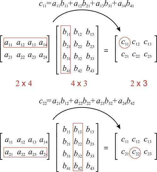
\(\newcommand{\avec}{\mathbf a}\) \(\newcommand{\bvec}{\mathbf b}\) \(\newcommand{\cvec}{\mathbf c}\) \(\newcommand{\dvec}{\mathbf d}\) \(\newcommand{\dtil}{\widetilde{\mathbf d}}\) \(\newcommand{\evec}{\mathbf e}\) \(\newcommand{\fvec}{\mathbf f}\) \(\newcommand{\nvec}{\mathbf n}\) \(\newcommand{\pvec}{\mathbf p}\) \(\newcommand{\qvec}{\mathbf q}\) \(\newcommand{\svec}{\mathbf s}\) \(\newcommand{\tvec}{\mathbf t}\) \(\newcommand{\uvec}{\mathbf u}\) \(\newcommand{\vvec}{\mathbf v}\) \(\newcommand{\wvec}{\mathbf w}\) \(\newcommand{\xvec}{\mathbf x}\) \(\newcommand{\yvec}{\mathbf y}\) \(\newcommand{\zvec}{\mathbf z}\) \(\newcommand{\rvec}{\mathbf r}\) \(\newcommand{\mvec}{\mathbf m}\) \(\newcommand{\zerovec}{\mathbf 0}\) \(\newcommand{\onevec}{\mathbf 1}\) \(\newcommand{\real}{\mathbb R}\) \(\newcommand{\twovec}[2]{\left[\begin{array}{r}#1 \\ #2 \end{array}\right]}\) \(\newcommand{\ctwovec}[2]{\left[\begin{array}{c}#1 \\ #2 \end{array}\right]}\) \(\newcommand{\threevec}[3]{\left[\begin{array}{r}#1 \\ #2 \\ #3 \end{array}\right]}\) \(\newcommand{\cthreevec}[3]{\left[\begin{array}{c}#1 \\ #2 \\ #3 \end{array}\right]}\) \(\newcommand{\fourvec}[4]{\left[\begin{array}{r}#1 \\ #2 \\ #3 \\ #4 \end{array}\right]}\) \(\newcommand{\cfourvec}[4]{\left[\begin{array}{c}#1 \\ #2 \\ #3 \\ #4 \end{array}\right]}\) \(\newcommand{\fivevec}[5]{\left[\begin{array}{r}#1 \\ #2 \\ #3 \\ #4 \\ #5 \\ \end{array}\right]}\) \(\newcommand{\cfivevec}[5]{\left[\begin{array}{c}#1 \\ #2 \\ #3 \\ #4 \\ #5 \\ \end{array}\right]}\) \(\newcommand{\mattwo}[4]{\left[\begin{array}{rr}#1 \amp #2 \\ #3 \amp #4 \\ \end{array}\right]}\) \(\newcommand{\laspan}[1]{\text{Span}\{#1\}}\) \(\newcommand{\bcal}{\cal B}\) \(\newcommand{\ccal}{\cal C}\) \(\newcommand{\scal}{\cal S}\) \(\newcommand{\wcal}{\cal W}\) \(\newcommand{\ecal}{\cal E}\) \(\newcommand{\coords}[2]{\left\{#1\right\}_{#2}}\) \(\newcommand{\gray}[1]{\color{gray}{#1}}\) \(\newcommand{\lgray}[1]{\color{lightgray}{#1}}\) \(\newcommand{\rank}{\operatorname{rank}}\) \(\newcommand{\row}{\text{Row}}\) \(\newcommand{\col}{\text{Col}}\) \(\renewcommand{\row}{\text{Row}}\) \(\newcommand{\nul}{\text{Nul}}\) \(\newcommand{\var}{\text{Var}}\) \(\newcommand{\corr}{\text{corr}}\) \(\newcommand{\len}[1]{\left|#1\right|}\) \(\newcommand{\bbar}{\overline{\bvec}}\) \(\newcommand{\bhat}{\widehat{\bvec}}\) \(\newcommand{\bperp}{\bvec^\perp}\) \(\newcommand{\xhat}{\widehat{\xvec}}\) \(\newcommand{\vhat}{\widehat{\vvec}}\) \(\newcommand{\uhat}{\widehat{\uvec}}\) \(\newcommand{\what}{\widehat{\wvec}}\) \(\newcommand{\Sighat}{\widehat{\Sigma}}\) \(\newcommand{\lt}{<}\) \(\newcommand{\gt}{>}\) \(\newcommand{\amp}{&}\) \(\definecolor{fillinmathshade}{gray}{0.9}\)If \(\mathbf{A}\) has dimensions \(m\times n\) and \(\mathbf{B}\) has dimensions \(n\times p\), then the product \(\mathbf{AB}\) is defined, and has dimensions \(m\times p\).
The entry \((ab)_{ij}\) is obtained by multiplying row \(i\) of \(\mathbf{A}\) by column \(j\) of \(\mathbf{B}\), which is done by multiplying corresponding entries together and then adding the results:
Calculate the product
\[\begin{pmatrix} 1 &-2 &4 \\ 5 &0 &3 \\ 0 & 1/2 &9 \end{pmatrix}\begin{pmatrix} 1 &0 \\ 5 &3 \\ -1 &0 \end{pmatrix} \nonumber\]
Solution
We need to multiply a \(3\times 3\) matrix by a \(3\times 2\) matrix, so we expect a \(3\times 2\) matrix as a result.
\[\begin{pmatrix} 1 &-2 &4 \\ 5 &0 &3 \\ 0 & 1/2 &9 \end{pmatrix}\begin{pmatrix} 1 &0 \\ 5 &3 \\ -1 &0 \end{pmatrix}=\begin{pmatrix} a&b \\ c&d \\ e &f \end{pmatrix} \nonumber\]
To calculate \(a\), which is entry (1,1), we use row 1 of the matrix on the left and column 1 of the matrix on the right:
\[\begin{pmatrix} {\color{red}1} &{\color{red}-2} &{\color{red}4} \\ 5 &0 &3 \\ 0 & 1/2 &9 \end{pmatrix}\begin{pmatrix} {\color{red}1} &0 \\ {\color{red}5} &3 \\ {\color{red}-1} &0 \end{pmatrix}=\begin{pmatrix} {\color{red}a}&b \\ c&d \\ e &f \end{pmatrix}\rightarrow a=1\times 1+(-2)\times 5+4\times (-1)=-13 \nonumber\]
To calculate \(b\), which is entry (1,2), we use row 1 of the matrix on the left and column 2 of the matrix on the right:
\[\begin{pmatrix} {\color{red}1} &{\color{red}-2} &{\color{red}4} \\ 5 &0 &3 \\ 0 & 1/2 &9 \end{pmatrix}\begin{pmatrix} 1&{\color{red}0} \\ 5&{\color{red}3} \\ -1&{\color{red}0} \end{pmatrix}=\begin{pmatrix} a&{\color{red}b} \\ c&d \\ e &f \end{pmatrix}\rightarrow b=1\times 0+(-2)\times 3+4\times 0=-6 \nonumber\]
To calculate \(c\), which is entry (2,1), we use row 2 of the matrix on the left and column 1 of the matrix on the right:
\[\begin{pmatrix} 1&-2&4\\ {\color{red}5} &{\color{red}0} &{\color{red}3} \\ 0 & 1/2 &9 \end{pmatrix}\begin{pmatrix} {\color{red}1} &0 \\ {\color{red}5} &3 \\ {\color{red}-1} &0 \end{pmatrix}=\begin{pmatrix} a&b \\ {\color{red}c}&d \\ e &f \end{pmatrix}\rightarrow c=5\times 1+0\times 5+3\times (-1)=2 \nonumber\]
To calculate \(d\), which is entry (2,2), we use row 2 of the matrix on the left and column 2 of the matrix on the right:
\[\begin{pmatrix} 1&-2&4\\ {\color{red}5} &{\color{red}0} &{\color{red}3} \\ 0 & 1/2 &9 \end{pmatrix}\begin{pmatrix} 1&{\color{red}0} \\ 5&{\color{red}3} \\ -1&{\color{red}0} \end{pmatrix}=\begin{pmatrix} a&b \\ c&{\color{red}d} \\ e &f \end{pmatrix}\rightarrow d=5\times 0+0\times 3+3\times 0=0 \nonumber\]
To calculate \(e\), which is entry (3,1), we use row 3 of the matrix on the left and column 1 of the matrix on the right:
\[\begin{pmatrix} 1&-2&4\\ 5&0&3 \\ {\color{red}0} &{\color{red}1/2} &{\color{red}9} \end{pmatrix}\begin{pmatrix} {\color{red}1} &0 \\ {\color{red}5} &3 \\ {\color{red}-1} &0 \end{pmatrix}=\begin{pmatrix} a&b \\ c&d \\ {\color{red}e} &f \end{pmatrix}\rightarrow e=0\times 1+1/2\times 5+9\times (-1)=-13/2 \nonumber\]
To calculate \(f\), which is entry (3,2), we use row 3 of the matrix on the left and column 2 of the matrix on the right:
\[\begin{pmatrix} 1&-2&4\\ 5&0&3 \\ {\color{red}0} &{\color{red}1/2} &{\color{red}9} \end{pmatrix}\begin{pmatrix} 1&{\color{red}0} \\ 5&{\color{red}3} \\ -1&{\color{red}0} \end{pmatrix}=\begin{pmatrix} a&b \\ c&d \\ e&{\color{red}f} \end{pmatrix}\rightarrow f=0\times 0+1/2\times 3+9\times 0=3/2 \nonumber\]
The result is:
\[\displaystyle{\color{Maroon}\begin{pmatrix} 1 &-2 &4 \\ 5 &0 &3 \\ 0 & 1/2 &9 \end{pmatrix}\begin{pmatrix} 1 &0 \\ 5 &3 \\ -1 &0 \end{pmatrix}=\begin{pmatrix} -13&-6 \\ 2&0 \\ -13/2 &3/2 \end{pmatrix}} \nonumber\]
Calculate
\[\begin{pmatrix} 1 &-2 &4 \\ 5 &0 &3 \\ \end{pmatrix}\begin{pmatrix} 1 \\ 5 \\ -1 \end{pmatrix}\nonumber\]
Solution
We are asked to multiply a \(2\times 3\) matrix by a \(3\times 1\) matrix (a column vector). The result will be a \(2\times 1\) matrix (a vector).
\[\begin{pmatrix} 1 &-2 &4 \\ 5 &0 &3 \\ \end{pmatrix}\begin{pmatrix} 1 \\ 5 \\ -1 \end{pmatrix}=\begin{pmatrix} a \\ b \end{pmatrix}\nonumber\]
\[a=1\times1+(-2)\times 5+ 4\times (-1)=-13\nonumber\]
\[b=5\times1+0\times 5+ 3\times (-1)=2\nonumber\]
The solution is:
\[\displaystyle{\color{Maroon}\begin{pmatrix} 1 &-2 &4 \\ 5 &0 &3 \\ \end{pmatrix}\begin{pmatrix} 1 \\ 5 \\ -1 \end{pmatrix}=\begin{pmatrix} -13 \\ 2 \end{pmatrix}}\nonumber\]
Need help? The link below contains solved examples: Multiplying matrices of different shapes (three examples): http://tinyurl.com/kn8ysqq
External links:
- Multiplying matrices, example 1: http://patrickjmt.com/matrices-multiplying-a-matrix-by-another-matrix/
- Multiplying matrices, example 2: http://patrickjmt.com/multiplying-matrices-example-2/
- Multiplying matrices, example 3: http://patrickjmt.com/multiplying-matrices-example-3/
The Commutator
Matrix multiplication is not, in general, commutative. For example, we can perform
\[\begin{pmatrix} 1 &-2 &4 \\ 5 &0 &3 \\ \end{pmatrix}\begin{pmatrix} 1 \\ 5 \\ -1 \end{pmatrix}=\begin{pmatrix} -13 \\ 2 \end{pmatrix} \nonumber\]
but cannot perform
\[\begin{pmatrix} 1 \\ 5 \\ -1 \end{pmatrix}\begin{pmatrix} 1 &-2 &4 \\ 5 &0 &3 \\ \end{pmatrix} \nonumber\]
Even with square matrices, that can be multiplied both ways, multiplication is not commutative. In this case, it is useful to define the commutator, defined as:
\[[\mathbf{A},\mathbf{B}]=\mathbf{A}\mathbf{B}-\mathbf{B}\mathbf{A} \nonumber\]
Given \(\mathbf{A}=\begin{pmatrix} 3&1 \\ 2&0 \end{pmatrix}\) and \(\mathbf{B}=\begin{pmatrix} 1&0 \\ -1&2 \end{pmatrix}\)
Calculate the commutator \([\mathbf{A},\mathbf{B}]\)
Solution
\[[\mathbf{A},\mathbf{B}]=\mathbf{A}\mathbf{B}-\mathbf{B}\mathbf{A}\nonumber\]
\[\mathbf{A}\mathbf{B}=\begin{pmatrix} 3&1 \\ 2&0 \end{pmatrix}\begin{pmatrix} 1&0 \\ -1&2 \end{pmatrix}=\begin{pmatrix} 3\times 1+1\times (-1)&3\times 0 +1\times 2 \\ 2\times 1+0\times (-1)&2\times 0+ 0\times 2 \end{pmatrix}=\begin{pmatrix} 2&2 \\ 2&0 \end{pmatrix}\nonumber\]
\[\mathbf{B}\mathbf{A}=\begin{pmatrix} 1&0 \\ -1&2 \end{pmatrix}\begin{pmatrix} 3&1 \\ 2&0 \end{pmatrix}=\begin{pmatrix} 1\times 3+0\times 2&1\times 1 +0\times 0 \\ -1\times 3+2\times 2&-1\times 1+2\times 0 \end{pmatrix}=\begin{pmatrix} 3&1 \\ 1&-1 \end{pmatrix}\nonumber\]
\[[\mathbf{A},\mathbf{B}]=\mathbf{A}\mathbf{B}-\mathbf{B}\mathbf{A}=\begin{pmatrix} 2&2 \\ 2&0 \end{pmatrix}-\begin{pmatrix} 3&1 \\ 1&-1 \end{pmatrix}=\begin{pmatrix} -1&1 \\ 1&1 \end{pmatrix}\nonumber\]
\[\displaystyle{\color{Maroon}[\mathbf{A},\mathbf{B}]=\begin{pmatrix} -1&1 \\ 1&1 \end{pmatrix}}\nonumber\]
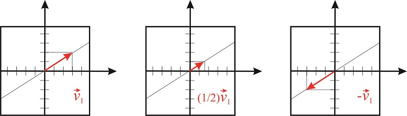
Multiplication of a vector by a scalar
The multiplication of a vector \(\vec{v_1}\) by a scalar \(n\) produces another vector of the same dimensions that lies in the same direction as \(\vec{v_1}\);
\[n\begin{pmatrix} x \\ y \end{pmatrix}=\begin{pmatrix} nx \\ ny \end{pmatrix} \nonumber\]
The scalar can stretch or compress the length of the vector, but cannot rotate it (figure [fig:vector_by_scalar]).
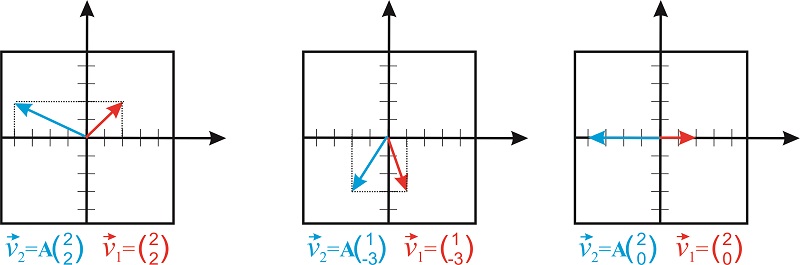
Multiplication of a square matrix by a vector
The multiplication of a vector \(\vec{v_1}\) by a square matrix produces another vector of the same dimensions of \(\vec{v_1}\). For example, we can multiply a \(2\times 2\) matrix and a 2-dimensional vector:
\[\begin{pmatrix} a&b \\ c&d \end{pmatrix}\begin{pmatrix} x \\ y \end{pmatrix}=\begin{pmatrix} ax+by \\ cx+dy \end{pmatrix} \nonumber\]
For example, consider the matrix
\[\mathbf{A}=\begin{pmatrix} -2 &0 \\ 0 &1 \end{pmatrix} \nonumber\]
The product
\[\begin{pmatrix} -2&0 \\ 0&1 \end{pmatrix}\begin{pmatrix} x \\ y \end{pmatrix} \nonumber\]
is
\[\begin{pmatrix} -2x \\ y \end{pmatrix} \nonumber\]
We see that \(2\times 2\) matrices act as operators that transform one 2-dimensional vector into another 2-dimensional vector. This particular matrix keeps the value of \(y\) constant and multiplies the value of \(x\) by -2 (Figure \(\PageIndex{3}\)).
Notice that matrices are useful ways of representing operators that change the orientation and size of a vector. An important class of operators that are of particular interest to chemists are the so-called symmetry operators.