2.7: The Maxwell Distribution Laws
- Page ID
- 41409
\( \newcommand{\vecs}[1]{\overset { \scriptstyle \rightharpoonup} {\mathbf{#1}} } \)
\( \newcommand{\vecd}[1]{\overset{-\!-\!\rightharpoonup}{\vphantom{a}\smash {#1}}} \)
\( \newcommand{\id}{\mathrm{id}}\) \( \newcommand{\Span}{\mathrm{span}}\)
( \newcommand{\kernel}{\mathrm{null}\,}\) \( \newcommand{\range}{\mathrm{range}\,}\)
\( \newcommand{\RealPart}{\mathrm{Re}}\) \( \newcommand{\ImaginaryPart}{\mathrm{Im}}\)
\( \newcommand{\Argument}{\mathrm{Arg}}\) \( \newcommand{\norm}[1]{\| #1 \|}\)
\( \newcommand{\inner}[2]{\langle #1, #2 \rangle}\)
\( \newcommand{\Span}{\mathrm{span}}\)
\( \newcommand{\id}{\mathrm{id}}\)
\( \newcommand{\Span}{\mathrm{span}}\)
\( \newcommand{\kernel}{\mathrm{null}\,}\)
\( \newcommand{\range}{\mathrm{range}\,}\)
\( \newcommand{\RealPart}{\mathrm{Re}}\)
\( \newcommand{\ImaginaryPart}{\mathrm{Im}}\)
\( \newcommand{\Argument}{\mathrm{Arg}}\)
\( \newcommand{\norm}[1]{\| #1 \|}\)
\( \newcommand{\inner}[2]{\langle #1, #2 \rangle}\)
\( \newcommand{\Span}{\mathrm{span}}\) \( \newcommand{\AA}{\unicode[.8,0]{x212B}}\)
\( \newcommand{\vectorA}[1]{\vec{#1}} % arrow\)
\( \newcommand{\vectorAt}[1]{\vec{\text{#1}}} % arrow\)
\( \newcommand{\vectorB}[1]{\overset { \scriptstyle \rightharpoonup} {\mathbf{#1}} } \)
\( \newcommand{\vectorC}[1]{\textbf{#1}} \)
\( \newcommand{\vectorD}[1]{\overrightarrow{#1}} \)
\( \newcommand{\vectorDt}[1]{\overrightarrow{\text{#1}}} \)
\( \newcommand{\vectE}[1]{\overset{-\!-\!\rightharpoonup}{\vphantom{a}\smash{\mathbf {#1}}}} \)
\( \newcommand{\vecs}[1]{\overset { \scriptstyle \rightharpoonup} {\mathbf{#1}} } \)
\( \newcommand{\vecd}[1]{\overset{-\!-\!\rightharpoonup}{\vphantom{a}\smash {#1}}} \)
\(\newcommand{\avec}{\mathbf a}\) \(\newcommand{\bvec}{\mathbf b}\) \(\newcommand{\cvec}{\mathbf c}\) \(\newcommand{\dvec}{\mathbf d}\) \(\newcommand{\dtil}{\widetilde{\mathbf d}}\) \(\newcommand{\evec}{\mathbf e}\) \(\newcommand{\fvec}{\mathbf f}\) \(\newcommand{\nvec}{\mathbf n}\) \(\newcommand{\pvec}{\mathbf p}\) \(\newcommand{\qvec}{\mathbf q}\) \(\newcommand{\svec}{\mathbf s}\) \(\newcommand{\tvec}{\mathbf t}\) \(\newcommand{\uvec}{\mathbf u}\) \(\newcommand{\vvec}{\mathbf v}\) \(\newcommand{\wvec}{\mathbf w}\) \(\newcommand{\xvec}{\mathbf x}\) \(\newcommand{\yvec}{\mathbf y}\) \(\newcommand{\zvec}{\mathbf z}\) \(\newcommand{\rvec}{\mathbf r}\) \(\newcommand{\mvec}{\mathbf m}\) \(\newcommand{\zerovec}{\mathbf 0}\) \(\newcommand{\onevec}{\mathbf 1}\) \(\newcommand{\real}{\mathbb R}\) \(\newcommand{\twovec}[2]{\left[\begin{array}{r}#1 \\ #2 \end{array}\right]}\) \(\newcommand{\ctwovec}[2]{\left[\begin{array}{c}#1 \\ #2 \end{array}\right]}\) \(\newcommand{\threevec}[3]{\left[\begin{array}{r}#1 \\ #2 \\ #3 \end{array}\right]}\) \(\newcommand{\cthreevec}[3]{\left[\begin{array}{c}#1 \\ #2 \\ #3 \end{array}\right]}\) \(\newcommand{\fourvec}[4]{\left[\begin{array}{r}#1 \\ #2 \\ #3 \\ #4 \end{array}\right]}\) \(\newcommand{\cfourvec}[4]{\left[\begin{array}{c}#1 \\ #2 \\ #3 \\ #4 \end{array}\right]}\) \(\newcommand{\fivevec}[5]{\left[\begin{array}{r}#1 \\ #2 \\ #3 \\ #4 \\ #5 \\ \end{array}\right]}\) \(\newcommand{\cfivevec}[5]{\left[\begin{array}{c}#1 \\ #2 \\ #3 \\ #4 \\ #5 \\ \end{array}\right]}\) \(\newcommand{\mattwo}[4]{\left[\begin{array}{rr}#1 \amp #2 \\ #3 \amp #4 \\ \end{array}\right]}\) \(\newcommand{\laspan}[1]{\text{Span}\{#1\}}\) \(\newcommand{\bcal}{\cal B}\) \(\newcommand{\ccal}{\cal C}\) \(\newcommand{\scal}{\cal S}\) \(\newcommand{\wcal}{\cal W}\) \(\newcommand{\ecal}{\cal E}\) \(\newcommand{\coords}[2]{\left\{#1\right\}_{#2}}\) \(\newcommand{\gray}[1]{\color{gray}{#1}}\) \(\newcommand{\lgray}[1]{\color{lightgray}{#1}}\) \(\newcommand{\rank}{\operatorname{rank}}\) \(\newcommand{\row}{\text{Row}}\) \(\newcommand{\col}{\text{Col}}\) \(\renewcommand{\row}{\text{Row}}\) \(\newcommand{\nul}{\text{Nul}}\) \(\newcommand{\var}{\text{Var}}\) \(\newcommand{\corr}{\text{corr}}\) \(\newcommand{\len}[1]{\left|#1\right|}\) \(\newcommand{\bbar}{\overline{\bvec}}\) \(\newcommand{\bhat}{\widehat{\bvec}}\) \(\newcommand{\bperp}{\bvec^\perp}\) \(\newcommand{\xhat}{\widehat{\xvec}}\) \(\newcommand{\vhat}{\widehat{\vvec}}\) \(\newcommand{\uhat}{\widehat{\uvec}}\) \(\newcommand{\what}{\widehat{\wvec}}\) \(\newcommand{\Sighat}{\widehat{\Sigma}}\) \(\newcommand{\lt}{<}\) \(\newcommand{\gt}{>}\) \(\newcommand{\amp}{&}\) \(\definecolor{fillinmathshade}{gray}{0.9}\)In the context of the Kinetic Molecular Theory of Gases, a gas contains a large number of particles in rapid motions. Each particle has a different speed, and each collision between particles changes the speeds of the particles. An understanding of the properties of the gas requires an understanding of the distribution of particle speeds.
Many molecules, many velocities
At temperatures above absolute zero, all molecules are in motion. In the case of a gas, this motion consists of straight-line jumps whose lengths are quite great compared to the dimensions of the molecule. Although we can never predict the velocity of a particular individual molecule, the fact that we are usually dealing with a huge number of them allows us to know what fraction of the molecules have kinetic energies (and hence velocities) that lie within any given range.
The trajectory of an individual gas molecule consists of a series of straight-line paths interrupted by collisions. What happens when two molecules collide depends on their relative kinetic energies; in general, a faster or heavier molecule will impart some of its kinetic energy to a slower or lighter one. Two molecules having identical masses and moving in opposite directions at the same speed will momentarily remain motionless after their collision.
If we could measure the instantaneous velocities of all the molecules in a sample of a gas at some fixed temperature, we would obtain a wide range of values. A few would be zero, and a few would be very high velocities, but the majority would fall into a more or less well defined range. We might be tempted to define an average velocity for a collection of molecules, but here we would need to be careful: molecules moving in opposite directions have velocities of opposite signs. Because the molecules are in a gas are in random thermal motion, there will be just about as many molecules moving in one direction as in the opposite direction, so the velocity vectors of opposite signs would all cancel and the average velocity would come out to zero. Since this answer is not very useful, we need to do our averaging in a slightly different way.
The proper treatment is to average the squares of the velocities, and then take the square root of this value. The resulting quantity is known as the root mean square (RMS) velocity
\[ v_{rms} = \sqrt{\dfrac{\sum \nu^2}{n}}\]
where \(n\) is the number of molecules in the system. The formula relating the RMS velocity to the temperature and molar mass is surprisingly simple (derived below), considering the great complexity of the events it represents:
\[ v_{rms} = \sqrt{\dfrac{3RT}{M}} \label{rms1}\]
where
- \(M\) is the molar mass in kg mol–1, and
- \(R\) is gas constant.
Equation \(\ref{rms1}\) can also be expressed as
\[ v_{rms} = \sqrt{\dfrac{3k_bT}{m}} \label{rms2}\]
where
- \(m\) is the molecular mass in kg
- \(k_b\) is Boltzmann constant and is just the “gas constant per molecule" \[k_b = \dfrac{R}{N_a} = \dfrac{R}{6.02 \times 10^{23}}\]
Equation \(\ref{rms2}\) is just the per atom version of Equation \(\ref{rms1}\) which is expressed in terms of per mol. Either equation will work.
Example \(\PageIndex{1}\)
What is the \(v_{rms}\) of a nitrogen molecule at 300 K?
Solution
The molar mass of \(N_2\) is 28.01 g/mol. Substituting in the above equation and expressing R in energy units, we obtain
\[v^2 =\dfrac{(3)(8.31 \;J \; mol^{-1} \; K^{-1})(300\;K)}{28.01 \times 10^{-3}\; Kg \; mol^{-1}} = 2.67 \times 10^5 \; \dfrac{J}{Kg} \nonumber\]
Recalling the definition of the joule (1 J = 1 kg m2 s–2) and taking the square root,
\[ \bar{v} = \sqrt{ \left(2.67 \times 10^5\; \dfrac{\cancel{J}}{\cancel{Kg}}\right) \left( \dfrac{ 1 \;\cancel{kg}\; m^2\; s^{–2}}{ 1 \;\cancel{J }} \right)} = 517 \;m /s \nonumber \]
or
\[ 517\, \dfrac{\cancel{m}}{s} \left(\dfrac{1\; km}{10^3\; \cancel{m}} \right) \left(\dfrac{3600\; \cancel{s}}{1\; hr} \right) = 1860\; km/hr \nonumber \]
Comment: this is fast! The velocity of a rifle bullet is typically 300-500 m s–1; convert to common units to see the comparison for yourself. A simpler formula for estimating average molecular velocities than \(\ref{rms1}\) is
\[ v_{rms} =157 \sqrt{\dfrac{T}{M}} \nonumber \]
in which \(v\) is in units of meters/sec, \(T\) is the absolute temperature and \(M\) the molar mass in grams.
The Boltzmann Distribution
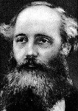
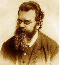
If we were to plot the number of molecules whose velocities fall within a series of narrow ranges, we would obtain a slightly asymmetric curve known as a velocity distribution. The peak of this curve would correspond to the most probable velocity. This velocity distribution curve is known as the Maxwell-Boltzmann distribution, but is frequently referred to only by Boltzmann's name. The Maxwell-Boltzmann distribution law was first worked out around 1850 by the great Scottish physicist, James Clerk Maxwell (left, 1831-1879), who is better known for discovering the laws of electromagnetic radiation. Later, the Austrian physicist Ludwig Boltzmann (1844-1906) put the relation on a sounder theoretical basis and simplified the mathematics somewhat. Boltzmann pioneered the application of statistics to the physics and thermodynamics of matter, and was an ardent supporter of the atomic theory of matter at a time when it was still not accepted by many of his contemporaries.
The Maxwell-Boltzmann distribution is used to determine how many molecules are moving between velocities \(v\) and \(v + dv\). Assuming that the one-dimensional distributions are independent of one another, that the velocity in the y and z directions does not affect the x velocity, for example, the Maxwell-Boltzmann distribution is given by
\[ \large \dfrac{dN}{N} = \left(\dfrac{m}{2\pi k_bT} \right)^{1/2}exp\left [\dfrac{-mv^2}{2k_b T}\right] dv \label{1}\]
where
- \(dN/N\) is the fraction of molecules moving at velocity \(v\) to \(v + dv\),
- \(m\) is the mass of the molecule,
- \(k_b\) is the Boltzmann constant, and
- \(T\) is the absolute temperature.1
Additionally, the function can be written in terms of the scalar quantity speed \(v\) instead of the vector quantity velocity. This form of the function defines the distribution of the gas molecules moving at different speeds, between \(v_1\) and \(v_2\), thus
\[f(v)=4\pi v^2 \left (\dfrac{m}{2\pi k_b T} \right)^{3/2}exp\left [\frac{-mv^2}{2k_bT}\right] \label{2}\]
Finally, the Maxwell-Boltzmann distribution can be used to determine the distribution of the kinetic energy of for a set of molecules. The distribution of the kinetic energy is identical to the distribution of the speeds for a certain gas at any temperature.2 The Maxwell-Boltzmann distribution is a probability distribution and just like any such distribution, can be characterized in a variety of ways including.
- Average Speed: The average speed is the sum of the speeds of all of the particles divided by the number of particles.
- Most Probable Speed: The most probable speed is the speed associated with the highest point in the Maxwell distribution. Only a small fraction of particles might have this speed, but it is more likely than any other speed.
- Width of the Distribution: The width of the distribution characterizes the most likely range of speeds for the particles. One measure of the width is the Full Width at Half Maximum (FWHM). To determine this value, find the height of the distribution at the most probable speed (this is the maximum height of the distribution). Divide the maximum height by two to obtain the half height, and locate the two speeds in the distribution that have this half-height value. On speed will be greater than the most probably speed and the other speed will be smaller. The full width is the difference between the two speeds at the half-maximum value.
Velocity distributions depend on temperature and mass
Higher temperatures allow a larger fraction of molecules to acquire greater amounts of kinetic energy, causing the Boltzmann plots to spread out. Figure \(\PageIndex{2}\) shows how the Maxwell-Boltzmann distribution is affected by temperature. At lower temperatures, the molecules have less energy. Therefore, the speeds of the molecules are lower and the distribution has a smaller range. As the temperature of the molecules increases, the distribution flattens out. Because the molecules have greater energy at higher temperature, the molecules are moving faster.
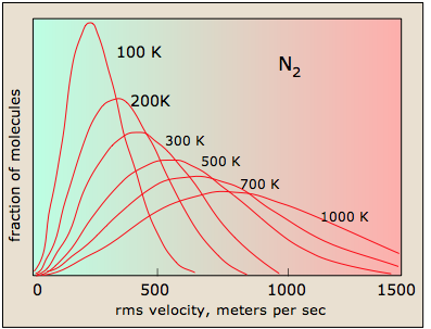
Notice how the left ends of the plots are anchored at zero velocity (there will always be a few molecules that happen to be at rest.) As a consequence, the curves flatten out as the higher temperatures make additional higher-velocity states of motion more accessible. The area under each plot is the same for a constant number of molecules.
All molecules have the same kinetic energy (mv2/2) at the same temperature, so the fraction of molecules with higher velocities will increase as m, and thus the molecular weight, decreases. Figure \(\PageIndex{3}\) shows the dependence of the Maxwell-Boltzmann distribution on molecule mass. On average, heavier molecules move more slowly than lighter molecules. Therefore, heavier molecules will have a smaller speed distribution, while lighter molecules will have a speed distribution that is more spread out.
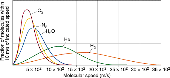
The Maxwell-Boltzmann equation, which forms the basis of the kinetic theory of gases, defines the distribution of speeds for a gas at a certain temperature. From this distribution function, the most probable speed, the average speed, and the root-mean-square speed can be derived.
Related Speed Expressions
Usually, we are more interested in the speeds of molecules rather than their component velocities. The Maxwell–Boltzmann distribution for the speed follows immediately from the distribution of the velocity vector, above. Note that the speed of an individual gas particle is:
\[v =\sqrt{v_x^2+ v_y^2 = v_z^2}\]
Three speed expressions can be derived from the Maxwell-Boltzmann distribution:
- the most probable speed,
- the average speed, and
- the root-mean-square speed.
The most probable speed is the maximum value on the distribution plot (Figure \(\PageIndex{4}\)}. This is established by finding the velocity when the derivative of Equation \(\ref{2}\) is zero
\[\dfrac{df(v)}{dv} = 0 \]
which is
\[\color{red} v_{mp}=\sqrt {\dfrac {2RT}{M}} \label{3a}\]
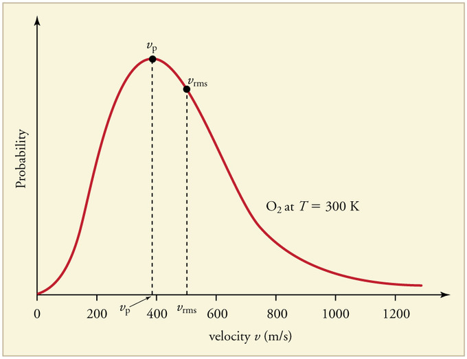
The average speed is the sum of the speeds of all the molecules divided by the number of molecules.
\[\color{red} v_{avg}= \bar{v} = \int_0^{\infty} v f(v) dv = \sqrt {\dfrac{8RT}{\pi M}} \label{3b}\]
The root-mean-square speed is square root of the average speed-squared.
\[ \color{red} v_{rms}= \bar{v^2} = \sqrt {\dfrac {3RT}{M}} \label{3c}\]
where
- \(R\) is the gas constant,
- \(T\) is the absolute temperature and
- \(M\) is the molar mass of the gas.
It always follows that for gases that follow the Maxwell-Boltzmann distribution:
\[v_{mp}< v_{avg}< v_{rms} \label{4}\]
Problems
- Using the Maxwell-Boltzman function, calculate the fraction of argon gas molecules with a speed of 305 m/s at 500 K.
- If the system in problem 1 has 0.46 moles of argon gas, how many molecules have the speed of 305 m/s?
- Calculate the values of \(C_{mp}\), \(C_{avg}\), and \(C_{rms}\) for xenon gas at 298 K.
- From the values calculated above, label the Boltzmann distribution plot (Figure 1) with the approximate locations of (C_{mp}\), \(C_{avg}\), and \(C_{rms}\).
- What will have a larger speed distribution, helium at 500 K or argon at 300 K? Helium at 300 K or argon at 500 K? Argon at 400 K or argon at 1000 K?
Answers
- 0.00141
- \(3.92 \times 10^{20}\) argon molecules
- cmp = 194.27 m/s, cavg = 219.21 m/s, crms = 237.93 m/s
- As stated above, Cmp is the most probable speed, thus it will be at the top of the distribution curve. To the right of the most probable speed will be the average speed, followed by the root-mean-square speed.
- Hint: Use the related speed expressions to determine the distribution of the gas molecules: helium at 500 K. helium at at 300 K. argon at 1000 K.
References
- Dunbar, R.C. Deriving the Maxwell Distribution J. Chem. Ed. 1982, 59, 22-23.
- Peckham, G.D.; McNaught, I.J.; Applications of the Maxwell-Boltzmann Distribution J. Chem. Ed. 1992, 69, 554-558.
- Chang, R. Physical Chemistry for the Biosciences, 25-27.
Contributors and Attributions
Stephen Lower, Professor Emeritus (Simon Fraser U.) Chem1 Virtual Textbook
- Adam Maley (Hope College)

