9.1: Prelude to Distance Measurements

At a distance of \(1 \mathrm{~nm}\) between two localized unpaired electrons, splitting \(\omega_{\perp}\) between the "horns" of the Pake pattern is about \(52 \mathrm{MHz}\) for two electron spins. Even strongly inhomogeneously broadened EPR spectra usually have features narrower than that (about \(2 \mathrm{mT}\) in a magnetic field sweep). Depending on the width of the narrowest features in the EPR spectrum and on availability of an experimental spectrum or realistic simulated spectrum in the absence of dipole-dipole coupling, distances up to \(1.5 \ldots 2.5 \mathrm{~nm}\) can be estimated from dipolar broadening by lineshape analysis. At distances below \(1.2 \mathrm{~nm}\), such analysis becomes uncertain due to the contribution from exchange coupling between the two electron spins, which cannot be computed by first principles and cannot be predicted with sufficient accuracy by quantum-chemical computations. If the two unpaired electrons are linked by a continuous chain of conjugated bonds, exchange coupling can be significant up to much longer distances.

Distance measurements are most valuable for spin labels or native paramagnetic centers in biomolecules or synthetic macromolecules and supramolecular assemblies. In such systems, if the two unpaired electrons are not linked by a \(\pi\)-electron system, exchange coupling is negligible with respect to dipole-dipole coupling for distances longer than \(1.5 \mathrm{~nm}\). Such systems can often assume different molecular conformations, i.e. their structure is not perfectly defined. Structural characterization thus profits strongly from the possibility to measure distance distributions on length scales that are comparable to the dimension of these systems. This dimension is of the order of 2 to \(20 \mathrm{~nm}\), corresponding to \(\omega_{\perp}\) between \(7 \mathrm{MHz}\) and \(7 \mathrm{kHz}\). In order to infer the distance distribution, this small dipole-dipole coupling needs to be separated from larger anisotropic interactions.

This separation of interactions is possible by observing the resonance frequency change for one spin in a pair (blue in Fig. 5.3) that is induced by flipping the spin of its coupling partner (red). In Fig. \(9.1\) the resonance frequency of the observer spin before the flip of its coupling partner is indicated by a dashed line. If the coupling partner is in its \(|\alpha\rangle\) state before the flip (left panel in Fig. 5.3), the local field at the observer spin will increase by \(\Delta B\) upon flipping the coupling partner. This causes an increase of the resonance frequency of the observer spin by the dipole-dipole coupling \(d\) (see Eq. (5.16)). If the coupling partner is in its \(|\beta\rangle\) state before the flip (right panel in Fig. 5.3), the local field at the observer spin will decrease by \(\Delta B\) upon flipping the coupling partner. This causes an decrease of the resonance frequency of the observer spin by the dipole-dipole coupling \(d\). In the high-temperature approximation, both these cases have the

Figure 9.1: Resonance frequency shift of an observer spin (blue transitions) by the change \(\pm \Delta B\) in local magnetic field that arises upon a flip of a second spin that is dipole-dipole coupled to the observer spin. Compare Fig. \(5.3\) for the local field picture.

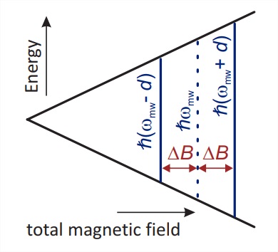
same probability. Hence, half of the observer spins will experience a frequency change \(+d\) and the other half will experience a frequency change \(-d\). If the observer spin evolves with changed frequency for some time \(t\), phases \(\pm d t\) will be gained compared to the situation without flipping the coupling partner. The additional phase can be observed as a cosine modulation \(\cos (d t)\) for both cases, as the cosine is an even function.