1.3: images

• delmar / Notes / EPR_PCIV_compressed
• D
• Export

1. Lecture Notes

2. Physical Chemistry IV

3. Part 2: Electron

Gunnar Jeschke

25

20

4. Copyright (c) 2016 Gunnar Jeschke

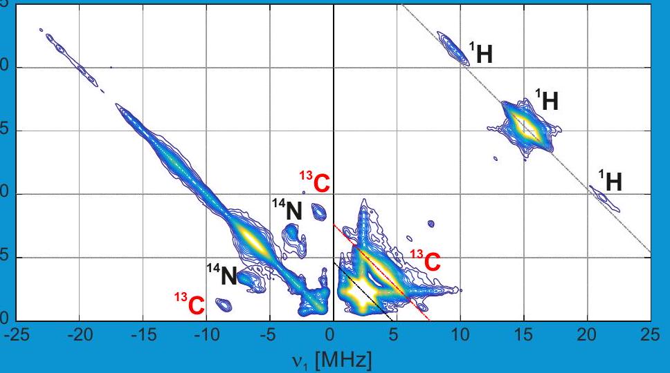
Title image: HYSCORE spectrum of a Ti(III) surface species (in collaboration with C. Copéret, F. Allouche, V. Kalendra)

Chapter 2 Stern-Gerlach memory plaque: Pen (GNU Free Documentation License)

Chapter 3 Zeeman effect on spectral lines (photograph by Pieter Zeeman, 1897)

Chapter 4 Hyperfine interaction by spin polarization (own work)

Chapter 5 Dipole-dipole interaction (own work)

Chapter 6 Energy level scheme of an spin system (own work)

Chapter 7 Field modulation in CW EPR (own work)

Chapter 8 Deuterium ESEEM trace of a spin-labelled protein (own work)

Chapter 9 Distance distribution measurement in a spin-labelled RNA construct (collaboration with O. Duss, M. Yulikov, F. H.-T. Allain)

Chapter 10 Electronic structure and molecular frame of a nitroxide spin label (own work)

5. PUBLISHED BY GUNNAR JESCHKE

http://WWW . epr. ethz . ch

Licensed under the Creative Commons Attribution-NonCommercial Unported License (the "License"). You may not use this file except in compliance with the License. You may obtain a copy of the License at http://creativecommons. org/licenses/by-nc/3.0.

Design and layout of the lecture notes are based on the Legrand Orange Book available at http://latextemplates. com/template/the-legrand-orange-book.

First printing, October 2016

6. Contents

Introduction

Electron spin

Magnetic resonance of the free electron

2.1.1 The magnetic moment of the free electron

2.2 Interactions in electron-nuclear spin systems 10

2.2.1 General consideration on spin interactions

2.2.2 The electron-nuclear spin Hamiltonian . . .......................... 12

3 Electron Zeeman Interaction .......................... 15

3.1 Physical origin of the shift 15

3.2 Electron Zeeman Hamiltonian 17

3.3 Spectral manifestation of the electron Zeeman interaction 18

3.3.1 Liquid solution

Solid state

Hyperfine Interaction

4.1 Physical origin of the hyperfine interaction 21

Fermi contact interaction

Spin polarization .................................... 23

4.2 Hyperfine Hamiltonian 24 4.3 Spectral manifestation of the hyperfine interaction 25

4.3.2 Liquid-solution nuclear frequency spectra

Solid-state EPR spectra ................................. 28

Solid-state nuclear frequency spectra

5 Electron-Electron Interactions .......................

5.1 Exchange interaction 31

Exchange Hamiltonian ................................... 32

5.1.3 Spectral manifestation of the exchange interaction . ....................

5.2 Dipole-dipole interaction 33

Physical picture

Dipole-dipole Hamiltonian

Spectral manifestation of the dipole-dipole interaction . . . . . . . . . . . . 35

5.3.1 Physical picture

6 Forbidden Electron-Nuclear Transitions . ................. 43

6.1 Physical picture 43

6.1.1 The

Local fields at the nuclear spin ........................................ 43

6.2 Product operator formalism with pseudo-secular interactions 45

Transformation of to the eigenbasis

6.2.2 General product operator computations for a non-diagonal Hamiltonian ......... 46

6.3 Generation and detection of nuclear coherence by electron spin excitation 47

Nuclear coherence generator

7 CW EPR Spectroscopy ................................ 49

7.1 Why and how CW EPR spectroscopy is done 49

7.1.1 Sensitivity advantages of CW EPR spectroscopy .........................................

7.1.3 Considerations on sample preparation

7.2 Theoretical description of CW EPR 53

8 Measurement of Small Hyperfine Couplings . .......... . . . 57

8.1 ENDOR 57

8.1.1 Advantages of electron-spin based detection of nuclear frequency spectra

8.1.2 Types of ENDOR experiments ............................ 57

8.1.3 Davies ENDOR 8.2 ESEEM and HYSCORE

8.2.1 ENDOR or ESEEM?

8.2.2 Three-pulse ESEEM

HYSCORE

Distance Distribution Measurements

9.1.1 The four-pulse DEER experiment

9.1.2 Sample requirements

9.2.1 Expression for the DEER signal

Background correction

9.2.3 Tikhonov regularization with non-negativity constraint . ................... 72

Spin Probes and Spin Traps

10.1.1 Spin probes and labels

Nitroxide radicals

The nitroxide EPR spectrum

Influence of dynamics on the nitroxide spectrum

Polarity and proticity

Water accessibility

Oxygen accessibility

Local measurements

Spin traps 83

Books 85

Articles 85

Index

7. 1 - Introduction

7.1. General Remarks

Electron Paramagnetic Resonance (EPR) spectroscopy is less well known and less widely applied than NMR spectroscopy. The reason is that EPR spectroscopy requires unpaired electrons and electron pairing is usually energetically favorable. Hence, only a small fraction of pure substances exhibit EPR signals, whereas NMR spectroscopy is applicable to almost any compound one can think of. On the other hand, as electron pairing underlies the chemical bond, unpaired electrons are associated with reactivity. Accordingly, EPR spectroscopy is a very important technique for understanding radical reactions, electron transfer processes, and transition metal catalysis, which are all related to the 'reactivity of the unpaired electron'. Some species with unpaired electrons are chemically stable and can be used as spin probes to study systems where NMR spectroscopy runs into resolution limits or cannot provide sufficient information for complete characterization of structure and dynamics. This lecture course introduces the basics for applying EPR spectroscopy on reactive or catalytically active species as well as on spin probes.

Many concepts in EPR spectroscopy are related to similar concepts in NMR spectroscopy. Hence, the lectures on EPR spectroscopy build on material that has been introduced before in the lectures on NMR spectroscopy. This material is briefly repeated and enhanced in this script and similarities as well as differences are pointed out. Such a linked treatment of the two techniques is not found in introductory textbooks. By emphasizing this link, the course emphasizes understanding of the physics that underlies NMR and EPR spectroscopy instead of focusing on individual application fields. We aim for understanding of spectra at a fundamental level and for understanding how parameters of the spin Hamiltonian can be measured with the best possible sensitivity and resolution.

Chapter 2 of the script introduces electron spin, relates it to nuclear spin, and discusses, which interactions contribute to the spin Hamiltonian of a paramagnetic system. Chapter 3 treats the electron Zeeman interaction, the deviation of the value of a bound electron from the value of a free electron, and the manifestation of anisotropy in solid-state EPR spectra. Chapter 4 introduces the hyperfine interaction between electron and nuclear spins, which provides most information on electronic and spatial structure of paramagnetic centers. Spectral manifestation in the liquid and solid state is considered for spectra of the electron spin and of the nuclear spins. Chapter 5 discusses phenomena that occur when the hyperfine interaction is so large that the high-field approximation is violated for the nuclear spin. In this situation, formally forbidden transitions become partially allowed and mixing of energy levels leads to changes in resonance frequencies. Chapter 6 discusses how the coupling between electron spins is described in the spin Hamiltonian, depending on its size. Throughout Chapters , the introduced interactions of the electron spin are related to electronic and spatial structure.

Chapter 7-9 are devoted to experimental techniques. In Chapter 7 , continuous-wave EPR is introduced as the most versatile and sensitive technique for measuring EPR spectra. The requirements for obtaining well resolved spectra with high signal-to-noise ratio are derived from first physical principles. Chapter 8 discusses two techniques for measuring hyperfine couplings in nuclear frequency spectra, where they are better resolved than in EPR spectra. Electron nuclear double resonance (ENDOR) experiments use electron spin polarization and detection of electron spins in order to enhance sensitivity of such measurements, but still rely on direct excitation of the nuclear spins. Electron spin echo envelope modulation (ESEEM) experiments rely on the forbidden electron-nuclear spin transitions discussed in Chapter 5. Chapter 9 treats the measurement of distance distributions in the nanometer range by separating the dipole-dipole coupling between electron spins from other interactions.

The final Chapter 10 introduces spin probing and spin trapping and, at the same time, demonstrates the application of concepts that were introduced in earlier Chapters.

At some points (dipole-dipole coupling, explanation of CW EPR spectroscopy in terms of the Bloch equations) this lecture script significantly overlaps with the NMR part of the lecture script. This is intended in order to make the EPR script reasonably self-contained. Note also that this lecture script serves two purposes. First, it should serve as a help in studying the subject and preparing for the examination. Second, it is reference material when you later encounter paramagnetic species in your own research and need to obtain information on them by EPR spectroscopy.

7.2. Suggested Reading & Electronic Resources

There is no textbook on EPR spectroscopy that treats all material of this course on a basic level. However, many of the concepts are covered by a title from the Oxford Chemistry Primer series by Chechik, Carter, and Murphy [CCM16]. Physically minded students may also appreciate the older standard textbook by Weil, Bolton, and Wertz [WBW94].

For some of the simulated spectra and worked examples in these lecture notes, Matlab scripts or Mathematica notebooks are provided on the lecture homepage. Part of the numerical simulations is based on EasySpin by Stefan Stoll (http://wWW. easyspin.org/) and another part on SPIDYAN by Stephan Pribitzer (http://www. epr . ethz. ch/software. html). Computations with product operator formalism require the Mathematica package SpinOp.m by Serge Boentges, which is available on the course homepage. An alternative larger package for such analytical computations is SpinDynamica by Malcolm Levitt (http://Www. spindynamica. soton. ac. uk/). Last, but not least the most extensive package for numerical simulations of magnetic resonance experiments is SPINACH by Ilya Kuprov et al. (http://spindynamics. org/ Spinach.php). For quantum-chemical computations of spin Hamiltonian parameters, the probably most versatile program is the freely available package ORCA (https://orcaforum . cec.mpg.de/).

8. Magnetic resonance of the free electron

The magnetic moment of the free electron Differences between EPR and NMR spectroscopy

Interactions in electron-nuclear spin systems General consideration on spin interactions The electron-nuclear spin Hamiltonian

9. 2 - Electron spin

10. Magnetic resonance of the free electron

10.2.1. The magnetic moment of the free electron

As an elementary particle, the electron has an intrinsic angular momentum called spin. The spin quantum number is , so that in an external magnetic field along , only two possible values can be observed for the component of this angular momentum, , corresponding to magnetic quantum number state and , corresponding to magnetic quantum number ( state . The energy difference between the corresponding two states of the electron results from the magnetic moment associated with spin. For a classical rotating particle with elementary charge , angular momentum and mass , this magnetic moment computes to

The charge-to-mass ratio is much larger for the electron than the corresponding ratio for a nucleus, where it is of the order of , where is the proton mass. By introducing the Bohr magneton and the quantum-mechanical correction factor , we can rewrite Eq. (2.1) as

Dirac-relativistic quantum mechanics provides , a correction that can also be found in a non-relativistic derivation. Exact measurements have shown that the value of a free electron deviates slightly from . The necessary correction can be derived by quantum electrodynamics, leading to . The energy difference between the two spin states of a free electron in an external magnetic field is given by

so that the gyromagnetic ratio of the free electron is . This gyromagnetic ratio corresponds to a resonance frequency of at a field of , which is by a factor of about 658 larger than the nuclear Zeeman frequency of a proton.

10.2.2. Differences between EPR and NMR spectroscopy

Most of the differences between NMR and EPR spectroscopy result from this much larger magnetic moment of the electron. Boltzmann polarization is larger by this factor and at the same magnetic field the detected photons have an energy larger by this factor. Relaxation times are roughly by a factor shorter, allowing for much faster repetition of EPR experiments compared to NMR experiments. As a result, EPR spectroscopy is much more sensitive. Standard instrumentation with an electromagnet working at a field of about and at microwave frequencies of about (X band) can detect about spins, if the sample has negligible dielectric microwave losses. In aqueous solution, organic radicals can be detected at concentrations down to in a measurement time of a few minutes.

Due to the large magnetic moment of the electron spin the high-temperature approximation may be violated without using exotic equipment. The spin transition energy of a free electron matches thermal energy at a temperature of and a field of about corresponding to a frequency of about (W band). Likewise, the high-field approximation may break down. The dipole-dipole interaction between two electron spins is by a factor of larger than between two protons and two unpaired electrons can come closer to each other than two protons. The zero-field splitting that results from such coupling can amount to a significant fraction of the electron Zeeman interaction or can even exceed it at the magnetic fields, where EPR experiments are usually performed . The hyperfine coupling between an electron and a nucleus can easily exceed the nuclear Zeeman frequency, which leads to breakdown of the high-field approximation for the nuclear spin.

11. Interactions in electron-nuclear spin systems

11.2.3. General consideration on spin interactions

Spins interact with magnetic fields. The interaction with a static external magnetic field is the Zeeman interaction, which is usually the largest spin interaction. At sufficiently large fields, where the high-field approximation holds, the Zeeman interaction determines the quantization direction of the spin. In this situation, is a good quantum number and, if the high-field approximation also holds for a nuclear spin , the magnetic quantum number is also a good quantum number. The energies of all spin levels can then be expressed by parameters that quantify spin interactions and by the magnetic quantum numbers. The vector of all magnetic quantum numbers defines the state of the spin system.

Spins also interact with the local magnetic fields induced by other spins. Usually, unpaired electrons are rare, so that each electron spin interacts with several nuclear spins in its vicinity, whereas each nuclear spin interacts with only one electron spin (Fig. 2.1). The hyperfine interaction between the electron and nuclear spin is usually much smaller than the electron Zeeman interaction, with exceptions for transition metal ions. In contrast, for nuclei in the close vicinity of the electron spin, the hyperfine interaction may be larger than the nuclear Zeeman interaction at the fields where EPR spectra are usually measured. In this case, which is discussed in Chapter 6, the high-field approximation breaks down and is not a good quantum number. Hyperfine couplings to nuclei are relevant as long as they are at least as large as the transverse relaxation rate of the coupled nuclear spin. Smaller couplings are unresolved.

In some systems, two or more unpaired electrons are so close to each other that their coupling exceeds their transverse relaxation rates . In fact, the isotropic part of this coupling can by far exceed the electron Zeeman interaction and often even thermal energy if two unpaired electrons reside in different molecular orbitals of the same organic molecule (triplet state molecule) or if several unpaired electrons belong to a high-spin state of a transition metal or rare earth metal ion. In this situation, the system is best described in a coupled representation with an

Figure 2.1: Scheme of interactions in electron-nuclear spin systems. All spins have a Zeeman interaction with the external magnetic field . Electron spins (red) interact with each other by the dipole-dipole interaction through space and by exchange due to overlap of the singly occupied molecular orbitals (green). Each electron spin interacts with nuclear spins (blue) in its vicinity by hyperfine couplings (purple). Couplings between nuclear spins are usually negligible in paramagnetic systems, as are chemical shifts. These two interactions are too small compared to the relaxation rate in the vicinity of an electron spin.

electron group spin . The isotropic coupling between the individual electron spins does not influence the sublevel splitting for a given group spin quantum number . The anisotropic coupling, which does lead to sublevel splitting, is called the zero-field or fine interaction. If the electron Zeeman interaction by far exceeds the spin-spin coupling, it is more convenient to describe the system in terms of the individual electron spins . The isotropic exchange coupling , which stems from overlap of two singly occupied molecular orbitals (SOMOs), then does contribute to level splitting. In addition, the dipole-dipole coupling through space between two electron spins also contributes.

Concept - Singly occupied molecular orbital (SOMO). Each molecular orbital can be occupied by two electrons with opposite magnetic spin quantum number . If a molecular orbital is singly occupied, the electron is unpaired and its magnetic spin quantum number can be changed by absorption or emission of photons. The orbital occupied by the unpaired electron is called a singly occupied molecular orbital (SOMO). Several unpaired electrons can exist in the same molecule or metal complex, i.e., there may be several SOMOs.

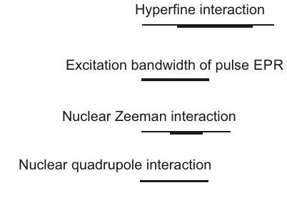
Nuclear spins in the vicinity of an electron spin relax much faster than nuclear spins in diamagnetic substances. Their transverse relaxation rates thus exceed couplings between nuclear spins and chemical shifts. These interactions, which are very important in NMR spectroscopy, are negligible in EPR spectroscopy. For nuclear spins no information on the chemical identity of a nucleus can be obtained, unless its hyperfine coupling is understood. The element can be identified via the nuclear Zeeman interaction. For nuclear spins , information on the chemical identity is encoded in the nuclear quadrupole interaction, whose magnitude usually exceeds .

An overview of all interactions and their typical magnitude in frequency units is given in Figure 2.2. This Figure also illustrates another difference between EPR and NMR spectroscopy. Several interactions, such as the zero-field interaction, the hyperfine interaction, larger dipole-dipole and exchange couplings between electron spins and also the anisotropy of the electron Zeeman interaction usually exceed the excitation bandwidth of the strongest and shortest microwave pulses

There is an exception. If the electron spin longitudinal relaxation rate exceeds the nuclear Zeeman interaction by far, nuclear spin relaxation is hardly affected by the presence of the electron spin. In this situation, EPR spectroscopy is impossible, however. that are available. NMR pulses sequences that rely on the ability to excite the full spectrum of a certain type of spins thus cannot easily be adapted to EPR spectroscopy.

11.2.4. The electron-nuclear spin Hamiltonian

Considering all interactions discussed in Section 2.2.1, the static spin Hamiltonian of an electron-nuclear spin system in angular frequency units can be written as

where index runs over all nuclear spins, indices and run over electron spins and the symbol denotes the transpose of a vector or vector operator. Often, only one electron spin and one nuclear spin have to be considered at once, so that the spin Hamiltonian simplifies drastically. For electron group spins , terms with higher powers of spin operators can be significant. We do not consider this complication here.

The electron Zeeman interaction is, in general, anisotropic and therefore parametrized by tensors . It is discussed in detail in Chapter 3 . In the nuclear Zeeman interaction , the nuclear Zeeman frequencies depend only on the element and isotope and thus can be specified without knowing electronic and spatial structure of the molecule. The hyperfine interaction is again anisotropic and thus characterized by tensors . It is discussed in detail in Chapter 4. All electron-electron interactions are explained in Chapter 5 . The zero-field interaction is purely anisotropic and thus characterized by traceless tensors . The exchange interaction is often purely isotropic and any anisotropic contribution cannot be experimentally distinguished from the purely anisotropic dipole-dipole interaction . Hence, the former interaction is characterized by scalars and the latter interaction by tensors . Finally, the nuclear quadrupole interaction is characterized by traceless tensors .

Electron Zeeman interaction

Zero field interaction

Dipole-dipole interaction

between weakly coupled electron spins

Homogeneous EPR linewidths

Figure 2.2: Relative magnitude of interactions that contribute to the Hamiltonian of electron-nuclear spin systems.

Physical origin of the shift Electron Zeeman Hamiltonian Spectral manifestation of the electron Zeeman interaction

Liquid solution Solid state

12. 3 - Electron Zeeman Interaction

13. Physical origin of the shift

Bound electrons are found to have values that differ from the value for the free electron. They depend on the orientation of the paramagnetic center with respect to the magnetic field vector . The main reason for this value shift is coupling of spin to orbital angular momentum of the electron. Spin-orbit coupling is a purely relativistic effect and is thus larger if orbitals of heavy atoms contribute to the SOMO. In most molecules, orbital angular momentum is quenched in the ground state. For this reason, SOC leads only to small or moderate shifts and can be treated as a perturbation. Such a perturbation treatment is not valid if the ground state is degenerate or near degenerate.

The perturbation treatment considers excited states where the unpaired electron is not in the SOMO of the ground state. Such excited states are slightly admixed to the ground state and the mixing arises from the orbital angular momentum operator. For simplicity, we consider a case where the main contribution to the shift arises from orbitals localized at a single, dominating atom and by single-electron SOC. To second order in perturbation theory, the matrix elements of the tensor can then be expressed as

where is a Kronecker delta, the factor in the shift term is the spin-orbit coupling constant for the dominating atom, and the matrix elements are computed as

where indices and run over the Cartesian directions , and . The operators , and are Cartesian components of the angular momentum operator, designates the orbital where the unpaired electron resides in an excited-state electron configuration, counted from for the SOMO of the ground state configuration. The energy of that orbital is .

Since the product of the overlap integrals in the numerator on the right-hand side of Eq. (3.2) is usually positive, the sign of the shift is determined by the denominator. The denominator is positive if a paired electron from a fully occupied orbital is promoted to the ground-state SOMO and negative if the unpaired electron is promoted to a previously unoccupied orbital (Figure Ground state

Excitation of a paired electron

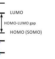
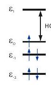
Figure 3.1: Admixture of excited states by orbital angular momentum operators leads to a shift by spin-orbit coupling. The energy difference in the perturbation expression is positive for excitation of a paired electron to the ground-state SOMO and negative for excitation of the paired electron to a higher energy orbital.

3.1). Because the energy gap between the SOMO and the lowest unoccupied orbital (LUMO) is usually larger than the one between occupied orbitals, terms with positive numerator dominate in the sum on the right-hand side of Eq. (3.2). Therefore, positive shifts are more frequently encountered than negative ones.

The relevant spin-orbit coupling constant depends on the element and type of orbital. It scales roughly with , where is the nuclear charge. Unless there is a very low lying excited state (near degeneracy of the ground state), contributions from heavy nuclei dominate. If their are none, as in organic radicals consisting of only hydrogen and second-row elements, shifts of only are observed, typical shifts are . Note that this still exceeds typical chemical shifts in NMR by one to two orders magnitude. For first-row transition metals, shifts are of the order of .

For rare-earth ions, the perturbation treatment breaks down. The Landé factor can then be computed from the term symbol for a doublet of levels

where is the quantum number for total angular momentum and the quantum number for orbital angular momentum. The principal values of the tensor are , and , where the with are differences between the eigenvalues of for the two levels.

If the structure of a paramagnetic center is known, the tensor can be computed by quantum chemistry. This works quite well for organic radicals and reasonably well for most first-row transition metal ions. Details are explained in [KBE04].

The tensor is a global property of the SOMO and is easily interpretable only if it is dominated by the contribution at a single atom, which is often, but not always, the case for transition metal and rare earth ion complexes. If the paramagnetic center has a symmetry axis with , the tensor has axial symmetry with principal values . For cubic or tetrahedral symmetry the value is isotropic, but not necessarily equal to . Isotropic values are also encountered to a very good approximation for transition metal and rare earth metal ions with half-filled shells, such as in Mn(II) complexes ( electron configuration) and Gd(III) complexes .

14. Electron Zeeman Hamiltonian

We consider a single electron spin and thus drop the sum and index in in Eq. (2.4). In the principal axes system (PAS) of the tensor, we can then express the electron Zeeman Hamiltonian as

where is the magnetic field, , and are the principal values of the tensor and the polar angles and determine the orientation of the magnetic field in the PAS.

This Hamiltonian is diagonalized by the Bleaney transformation, providing

with the effective value at orientation

If anisotropy of the tensor is significant, the axis in Eq. (3.5) is tilted from the direction of the magnetic field. This effect is negligible for most organic radicals, but not for transition metal ions or rare earth ions. Eq. (3.6) for the effective values describes an ellipsoid (Figure ).

Figure 3.2: Ellipsoid describing the orientation dependence of the effective value in the PAS of the tensor. At a given direction of the magnetic field vector (red), corresponds to distance between the origin and the point where intersects the ellipsoid surface.

Concept 3.2.1 - Energy levels in the high-field approximation. In the high-field approximation the energy contribution of a Hamiltonian term to the level with magnetic quantum numbers and can be computed by replacing the operators by the corresponding magnetic quantum numbers. This is because the magnetic quantum numbers are the eigenvalues of the operators, all operators commute with each other, and contributions with all other Cartesian spin operators are negligible in this approximation. For the electron Zeeman energy contribution is . If the high-field approximation is slightly violated, this expression corresponds to a first-order perturbation treatment. The selection rule for transitions in EPR spectroscopy is and it applies strictly as long as the high-field approximation applies strictly to all spins. This selection rule results from conservation of angular momentum on absorption of a microwave photon and from the fact that the microwave photon interacts with electron spin transitions. It follows that the first-order contribution of the electron Zeeman interaction to the frequencies of all electron spin transitions is the same, namely . As we shall see in Chapter 7 , EPR spectra are usually measured at constant microwave frequency by sweeping the magnetic field . The resonance field is then given by

For nuclear spin transitions, , the electron Zeeman interaction does not contribute to the transition frequency.

14.1. Spectral manifestation of the electron Zeeman interaction

14.1.1. Liquid solution

In liquid solution, molecules tumble due to Brownian rotational diffusion. The time scale of this motion can be characterized by a rotational correlation time that in non-viscous solvents is of the order of for small molecules, and of the order of to 100 ns for proteins and other macromolecules. For a globular molecule with radius in a solvent with viscosity , the rotational correlation time can be roughly estimated by the Stokes-Einstein law

If this correlation time and the maximum difference between the transition frequencies of any two orientations of the molecule in the magnetic field fulfill the relation , anisotropy is fully averaged and only the isotropic average of the transition frequencies is observed. For somewhat slower rotation, modulation of the transition frequency by molecular tumbling leads to line broadening as it shortens the transverse relaxation time . In the slow-tumbling regime, where , anisotropy is incompletely averaged and line width attains a maximum. For , the solid-state spectrum is observed. The phenomena can be described as a multi-site exchange between the various orientations of the molecule (see Section 10.1.4), which is analogous to the chemical exchange discussed in the NMR part of the lecture course.

For the electron Zeeman interaction, fast tumbling leads to an average resonance field

with the isotropic value . For small organic radicals in non-viscous solvents at X-band frequencies around , line broadening from anisotropy is negligible. At W-band frequencies of for organic radicals and already at X-band frequencies for small transition metal complexes, such broadening can be substantial. For large macromolecules or in viscous solvents, solid-state like EPR spectra can be observed in liquid solution.

14.1.2. Solid state

For a single-crystal sample, the resonance field at any given orientation can be computed by Eq. (3.7). Often, only microcrystalline powders are available or the sample is measured in glassy frozen solution. Under such conditions, all orientations contribute equally. With respect to the

Figure 3.3: Powder line shape for a tensor with axial symmetry. (a) The probability density to find an orientation with polar angle is proportional to the circumference of a circle a angle on a unit sphere. (b) Probability density . The effective value at angle is . (c) Schematic powder line shape. The pattern corresponds to for a field sweep and to for a frequency sweep. Because of the frame tilting, the isotropic value is not encountered at the magic angle, although the shift is small if .

polar angles, this implies that is uniformly distributed, whereas the probability to encounter a certain angle is proportional to (Figure 3.3). The line shape of the absorption spectrum is most easily understood for axial symmetry of the tensor. Transitions are observed only in the range between the limiting resonance fields at and . The spectrum has a global maximum at and a minimum at .

In CW EPR spectroscopy we do not observe the absorption line shape, but rather its first derivative (see Chapter 7). This derivative line shape has sharp features at the line shape singularities of the absorption spectrum and very weak amplitude in between (Figure ).

Concept 3.3.1 - Orientation selection. The spread of the spectrum of a powder sample or glassy frozen solution allows for selecting molecules with a certain orientation with respect to the magnetic field. For an axial tensor only orientations near the axis of the tensor PAS are selected when observing near the resonance field of . In contrast, when observing near the resonance field for , orientations withing the whole plane of the PAS contribute. For the case of orthorhombic symmetry with three distinct principal values , and , narrow sets of orientations can be observed at the resonance fields corresponding to the extreme values and (see right top panel in Figure 3.4). At the intermediate principal value a broad range of orientations contributes, because the same resonance field can be realized by orientations other than and . Such orientation selection can enhance the resolution of ENDOR and ESEEM spectra (Chapter 8) and simplify their interpretation. axial symmetry

orthorhombic

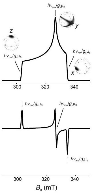
Figure 3.4: Simulated X-band EPR spectra for systems with only anisotropy. The upper panels show absorption spectra as they can be measured by echo-detected field-swept EPR spectroscopy. The lower panels show the first derivative of the absorption spectra as they are detected by continuous-wave EPR. The unit-sphere pictures in the right upper panel visualize the orientations that are selected at the resonance fields corresponding to the principal values of the tensor.

14.2. Physical origin of the hyperfine interaction

The magnetic moments of an electron and a nuclear spin couple by the magnetic dipole-dipole interaction; similar to the dipole-dipole interaction between nuclear spins discussed in the NMR part of the lecture course. The main difference to the NMR case is that, in many cases, a point-dipole description is not a good approximation for the electron spin, as the electron is distributed over the SOMO. The nucleus under consideration can be considered as well localized in space. We now picture the SOMO as a linear combination of atomic orbitals. Contributions from spin density in an atomic orbital of another nucleus (population of the unpaired electron in such an atomic orbital) can be approximated by assuming that the unpaired electron is a point-dipole localized at this other nucleus.

For spin density in atomic orbitals on the same nucleus, we have to distinguish between types of atomic orbitals. In orbitals, the unpaired electron has finite probability density for residing at the nucleus, at zero distance to the nuclear spin. This leads to a singularity of the dipole-dipole interaction, since this interaction scales with . The singularity has been treated by Fermi. The contribution to the hyperfine coupling from spin density in orbitals on the nucleus under consideration is therefor called Fermi contact interaction. Because of the spherical symmetry of orbitals, the Fermi contact interaction is purely isotropic.

For spin density in other orbitals ( orbitals) on the nucleus under consideration, the dipole-dipole interaction must be averaged over the spatial distribution of the electron spin in these orbitals. This average has no isotropic contribution. Therefore, spin density in orbitals does not influence spectra of fast tumbling radicals or metal complexes in liquid solution and neither does spin density in orbitals of other nuclei. The isotropic couplings detected in solution result only from the Fermi contact interaction.

Since the isotropic and purely anisotropic contributions to the hyperfine coupling have different physical origin, we separate these contributions in the hyperfine tensor that describes the interaction between electron spin and nuclear spin :

where is the isotropic hyperfine coupling and the purely anisotropic coupling. In the following, we drop the electron and nuclear spin indices and .

14.2.1. Dipole-dipole hyperfine interaction

The anisotropic hyperfine coupling tensor of a given nucleus can be computed from the ground state wavefunction by applying the correspondence principle to the classical interaction between two point dipoles

Such computations are implemented in quantum chemistry programs such as ORCA, ADF, or Gaussian. If the SOMO is considered as a linear combination of atomic orbitals, the contributions from an individual orbital can be expressed as the product of spin density in this orbital with a spatial factor that can be computed once for all. The spatial factors have been tabulated [KM85]. In general, nuclei of elements with larger electronegativity have larger spatial factors. At the same spatial factor, such as for isotopes of the same element, the hyperfine coupling is proportional to the nuclear value and thus proportional to the gyromagnetic ratio of the nucleus. Hence, a deuterium coupling can be computed from a known proton coupling or vice versa.

A special situation applies to protons, alkali metals and earth alkaline metals, which have no significant spin densities in , or -orbitals. In this case, the anisotropic contribution can only arise from through-space dipole-dipole coupling to centers of spin density at other nuclei. In a point-dipole approximation the hyperfine tensor is then given by

where the sum runs over all nuclei with significant spin density (summed over all orbitals at this nucleus) other than nucleus under consideration. The are distances between the nucleus under consideration and the centers of spin density, and the are unit vectors along the direction from the considered nucleus to the center of spin density. For protons in transition metal complexes it is often a good approximation to consider spin density only at the central metal ion. The distance from the proton to the central ion can then be directly inferred from the anisotropic part of the hyperfine coupling.

Hyperfine tensor contributions computed by any of these ways must be corrected for the influence of if the tensor is strongly anisotropic. If the dominant contribution to arises at a single nucleus, the hyperfine tensor at this nucleus can be corrected by

The product g may have an isotropic part, although is purely anisotropic. This isotropic pseudocontact contribution depends on the relative orientation of the tensor and the spin-only dipole-dipole hyperfine tensor . The correction is negligible for most organic radicals, but not for paramagnetic metal ions. If contributions to arise from several centers, the necessary correction cannot be written as a function of the tensor.

14.2.2. Fermi contact interaction

The Fermi contact contribution takes the form

Most literature holds that the correction should be done for all nuclei. As pointed out by Frank Neese, this is not true. An earlier discussion of this point is found in [Lef67] where is the spin density in the orbital under consideration, the nuclear value and the nuclear magneton . The factor denotes the probability to find the electron at this nucleus in the ground state with wave function and has been tabulated [KM85].

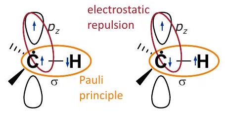
Figure 4.1: Transfer of spin density by the spin polarization mechanism. According to the Pauli principle, the two electrons in the C-H bond orbital must have opposite spin state. If the unpaired electron resides in a orbital on the atom, for other electrons on the same atom the same spin state is slightly favored, as this minimizes electrostatic repulsion. Hence, for the electron at the atom, the opposite spin state (left panel) is slightly favored over the same spin state (right panel). Positive spin density in the orbital on the atom induces some negative spin density in the orbital on the atom.

14.2.3. Spin polarization

The contributions to the hyperfine coupling discussed up to this point can be understood and computed in a single-electron picture. Further contributions arise from correlation of electrons in a molecule. Assume that the orbital on a carbon atom contributes to the SOMO, so that the spin state of the electron is preferred in that orbital (Fig. 4.1). Electrons in other orbitals on the same atom will then also have a slight preference for the state (left panel), as electrons with the same spin tend to avoid each other and thus have less electrostatic repulsion. In particular, this means that the spin configuration in the left panel of Fig. is slightly more preferable than the one in the right panel. According to the Pauli principle, the two electrons that share the bond orbital of the bond must have antiparallel spin. Thus, the electron in the orbital of the hydrogen atom that is bound to the spin-carrying carbon atom has a slight preference for the state. This corresponds to a negative isotropic hyperfine coupling of the directly bound proton, which is induced by the positive hyperfine coupling of the adjacent carbon atom. The effect is termed "spin polarization", although it has no physical relation to the polarization of electron spin transitions in an external magnetic field.

Spin polarization is important, as it transfers spin density from orbitals, where it is invisible in liquid solution and from carbon atoms with low natural abundance of the magnetic isotope to orbitals on protons, where it can be easily observed in liquid solution. This transfer occurs, both, in radicals, where the unpaired electron is localized on a single atom, and in radicals, where it is distributed over the system. The latter case is of larger interest, as the distribution of the orbital over the nuclei can be mapped by measuring and assigning the isotropic proton hyperfine couplings. This coupling can be predicted by the McConnell equation

where is the spin density at the adjacent carbon atom and is a parameter of the order of , which slightly depends on structure of the system.

This preference for electrons on the same atom to have parallel spin is also the basis of Hund's rule.

Figure 4.2: Mapping of the LUMO and HOMO of an aromatic molecule via measurements of hyperfine couplings after one-electron reduction or oxidation. Reduction leads to an anion radical, whose SOMO is a good approximation to the lowest unoccupied molecular orbital (LUMO) of the neutral parent molecule. Oxidation leads to an cation radical, whose SOMO is a good approximation to the highest occupied molecular orbital (HOMO) of the neutral parent molecule.

The McConnell equation is mainly applied for mapping the LUMO and HOMO of aromatic molecules (Figure 4.2). An unpaired electron can be put into these orbitals by one-electron reduction or oxidation, respectively, without perturbing the orbitals too strongly. The isotropic hyperfine couplings of the hydrogen atom directly bound to a carbon atom report on the contribution of the orbital of this carbon atom to the orbital. The challenges in this mapping are twofold. First, it is hard to assign the observed couplings to the hydrogen atoms unless a model for the distribution of the orbital is already available. Second, the method is blind to carbon atoms without a directly bonded hydrogen atom.

14.3. Hyperfine Hamiltonian

We consider the interaction of a single electron spin with a single nuclear spin and thus drop the sums and indices and in in Eq. (2.4). In general, all matrix elements of the hyperfine tensor will be non-zero after the Bleaney transformation to the frame where the electron Zeeman interaction is along the axis (see Eq. 3.5). The hyperfine Hamiltonian is then given by

Note that the axis of the nuclear spin coordinate system is parallel to the magnetic field vector whereas the one of the electron spin system is tilted, if anisotropy is significant. Hence, the hyperfine tensor is not a tensor in the strict mathematical sense, but rather an interaction matrix.

In Eq. (4.7), the term is secular and must always be kept. Usually, the high-field approximation does hold for the electron spin, so that all terms containing or operators are non-secular and can be dropped. The truncated hyperfine Hamiltonian thus reads

The first two terms on the right-hand side can be considered as defining an effective transverse coupling that is the sum of a vector with length along and a vector of length along . The length of the sum vector is . The truncated hyperfine Hamiltonian simplifies if we take the laboratory frame axis for the nuclear spin along the direction of this effective transverse hyperfine coupling. In this frame we have

where quantifies the secular hyperfine coupling and the pseudo-secular hyperfine coupling. The latter coupling must be considered if and only if the hyperfine coupling violates the high-field approximation for the nuclear spin (see Chapter 6).

If anisotropy is very small, as is the case for organic radicals, the axes of the two spin coordinate systems are parallel. In this situation and for a hyperfine tensor with axial symmetry, and can be expressed as

where is the angle between the static magnetic field and the symmetry axis of the hyperfine tensor and is the anisotropy of the hyperfine coupling. The principal values of the hyperfine tensor are and . The pseudo-secular contribution vanishes along the principal axes of the hyperfine tensor, where is either or or for a purely isotropic hyperfine coupling. Hence, the pseudo-secular contribution can also be dropped when considering fast tumbling radicals in the liquid state. We now consider the point-dipole approximation, where the electron spin is well localized on the length scale of the electron-nuclear distance and assume that arises solely from through-space interactions. This applies to hydrogen, alkali and earth alkali ions. We then find

For the moment we assume that the pseudo-secular contribution is either negligible or can be considered as a small perturbation. The other case is treated in Chapter 6 . To first order, the contribution of the hyperfine interaction to the energy levels is then given by . In the EPR spectrum, each nucleus with spin generates electron spin transitions with that can be labeled by the values of . In the nuclear frequency spectrum, each nucleus exhibits transitions with . For nuclear spins in the solid state, each transition is further split into transitions by the nuclear quadrupole interaction. The contribution of the secular hyperfine coupling to the electron transition frequencies is , whereas it is for nuclear transition frequencies. In both cases, the splitting between adjacent lines of a hyperfine multiplet is given by .

14.4. Spectral manifestation of the hyperfine interaction

14.4.1. Liquid-solution EPR spectra

Since each nucleus splits each electron spin transition into transitions with different frequencies, the number of EPR transitions is . Some of these transitions may coincide if hyperfine couplings are the same or integer multiples of each other. An important case, where hyperfine couplings are exactly the same are chemically equivalent nuclei. For instance, two nuclei can have spin state combinations , and . The contributions to the transition frequencies are , and

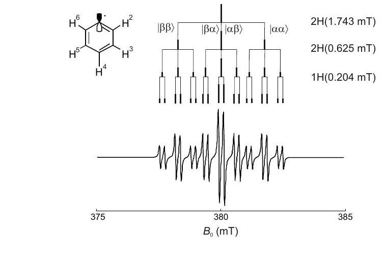
Figure 4.3: Hyperfine splitting in the EPR spectrum of the phenyl radical. The largest hyperfine coupling for the two equivalent ortho protons generates a triplet of lines with relative intensities . The medium coupling to the two equivalent meta proton splits each line again into a pattern, leading to 9 lines with an intensity ratio of . Finally, each line is split into a doublet by the small hyperfine coupling of the para proton, leading to 18 lines with intensity ratio .

. For equivalent nuclei with only three lines are observed with hyperfine shifts of , and with respect to the electron Zeeman frequency. The unshifted center line has twice the amplitude than the shifted lines, leading to a pattern with splitting . For equivalent nuclei with the number of lines is and the relative intensities can be inferred from Pascal's triangle. For a group of equivalent nuclei with arbitrary spin quantum number the number of lines is . The multiplicities of groups of equivalent nuclei multiply. Hence, the total number of EPR lines is

where index runs over the groups of equivalent nuclei.

Figure illustrates on the example of the phenyl radical how the multiplet pattern arises. For radicals with more extended systems, the number of lines can be very large and it may become impossible to fully resolve the spectrum. Even if the spectrum is fully resolved, analysis of the multiplet pattern may be a formidable task. An algorithm that works well for analysis of patterns with a moderate number of lines is given in [CCM16].

14.4.2. Liquid-solution nuclear frequency spectra

As mentioned in Section the secular hyperfine coupling can be inferred from nuclear frequency spectra as well as from EPR spectra. Line widths are smaller in the nuclear frequency spectra, since nuclear spins have longer transverse relaxation times . Another advantage of nuclear frequency spectra arises from the fact that the electron spin interacts with all nuclear spins whereas each nuclear spin interacts with only one electron spin (Figure 4.4). The number of lines in nuclear frequency spectra thus grows only linearly with the number of nuclei, whereas

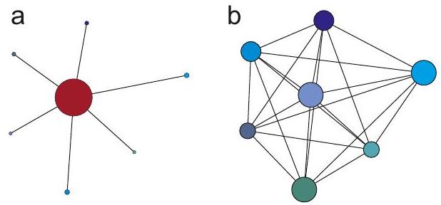
Figure 4.4: Topologies of an electron-nuclear spin system for EPR spectroscopy (a) and of a nuclear spin system typical for NMR spectroscopy (b). Because of the much larger magnetic moment of the electron spin, the electron spin "sees" all nuclei, while each nuclear spin in the EPR case sees only the electron spin. In the NMR case, each nuclear spin sees each other nuclear spin, giving rise to very rich, but harder to analyze information.

it grows exponentially in EPR spectra. In liquid solution, each group of equivalent nuclear spins adds lines, so that the number of lines for such groups is

The nuclear frequency spectra in liquid solution can be measured by CW ENDOR, a technique that is briefly discussed in Section 8.1.2.

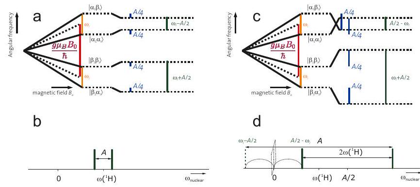
Figure 4.5: Energy level schemes (a,c) and nuclear frequency spectra (b,d) in the weak hyperfine coupling and strong hyperfine coupling (c,d) cases for an electron-nuclear spin system , . Here, is assumed to be negative and is assumed to be positive. (a) In the weak-coupling case, , the two nuclear spin transitions (green) have frequencies . (b) In the weak-coupling case, the doublet is centered at frequency and split by . (c) In the strong-coupling case, , levels cross for one of the electron spin states. The two nuclear spin transitions (green) have frequencies . (d) In the strong-coupling case, the doublet is centered at frequency and split by .

A complication in interpretation of nuclear frequency spectra can arise from the fact that the hyperfine interaction may be larger than the nuclear Zeeman interaction. This is illustrated in Figure 4.5. Only in the weak-coupling case with the hyperfine doublet in nuclear frequency spectra is centered at and split by . In the strong-coupling case, hyperfine sublevels cross for one of the electron spin states and the nuclear frequency becomes negative. As the sign of the frequency is not detected, the line is found at frequency instead, i.e., it is "mirrored" at the zero frequency. This results in a doublet centered at frequency and split by . Recognition of such cases in well resolved liquid-state spectra is simplified by the fact that the nuclear Zeeman frequency can only assume a few values that are known if the nuclear isotopes in the molecule and the magnetic field are known. Figure illustrates how the nuclear frequency spectrum of the phenyl radical is constructed based on such considerations. The spectrum has only 6 lines, compared to the 18 lines that arise in the EPR spectrum in Figure 4.3.

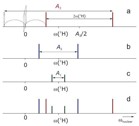
Figure 4.6: Schematic ENDOR (nuclear frequency) spectrum of the phenyl radical at an X-band frequency where . (a) Subspectrum of the two equivalent ortho protons. The strong-coupling case applies. (b) Subspectrum of the two equivalent meta protons. The weak-coupling case applies. (c) Subspectrum of the para proton. The weak-coupling case applies. (d) Complete spectrum.

14.4.3. Solid-state EPR spectra

In the solid state, construction of the EPR spectra is complicated by the fact that the electron Zeeman interaction is anisotropic. At each individual orientation of the molecule, the spectrum looks like the pattern in liquid state, but both the central frequency of the multiplet and the hyperfine splittings depend on orientation. As these frequency distributions are continuous, resolved splittings are usually observed only at the singularities of the line shape pattern of the interaction with the largest anisotropy. For organic radicals at X-band frequencies, often hyperfine anisotropy dominates. At high frequencies or for transition metal ions, often electron Zeeman anisotropy dominates. The exact line shape depends not only on the principal values of the tensor and the hyperfine tensors, but also on relative orientation of their PASs. The general case is complicated and requires numerical simulations, for instance, by EasySpin.

However, simple cases, where the hyperfine interaction of only one nucleus dominates and the PASs of the and hyperfine tensor coincide, are quite often encountered. For instance, Cu(II) complexes are often square planar and, if all four ligands are the same, have a symmetry axis. The tensor than has axial symmetry with the axis being the unique axis. The hyperfine tensors of and have the same symmetry and the same unique axis. The two isotopes both have spin and very similar gyromagnetic ratios. The spectra can thus be understood by considering one electron spin and one nuclear spin with axial and hyperfine tensors with a coinciding unique axis.

In this situation, the subspectra for each of the nuclear spin states , and take on a similar form as shown in Figure . The resonance field can be computed by solving

where is the angle between the symmetry axis and the magnetic field vector . The singularities are encountered at and and correspond to angular frequencies and .

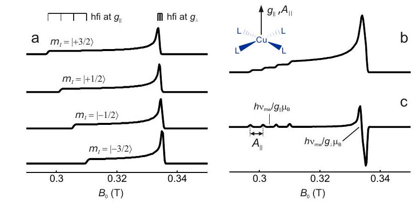
Figure 4.7: Construction of a solid-state EPR spectrum for a copper(II) complex with four equivalent ligands and square planar coordination. The and principal axes directions coincide with the symmetry axis of the complex (inset). (a) Subspectra for the four nuclear spin states with different magnetic spin quantum number . (b) Absorption spectrum. (c) Derivative of the absorption spectrum.

The construction of a Cu(II) EPR spectrum according to these considerations is shown in Figure 4.7. The values of and can be inferred by analyzing the singularities near the low-field edge of the spectrum. Near the high-field edge, the hyperfine splitting is usually not resolved. Here, corresponds to the maximum of the absorption spectrum and to the zero crossing of its derivative.

14.4.4. Solid-state nuclear frequency spectra

Again, a simpler situation is encountered in nuclear frequency spectra, as the nuclear Zeeman frequency is isotropic and chemical shift anisotropy is negligibly small compared to hyperfine anisotropy. Furthermore, resolution is much better for the reasons discussed above, so that smaller hyperfine couplings and anisotropies can be detected. If anisotropy of the hyperfine coupling is dominated by through-space dipole-dipole coupling to a single center of spin density, as is often the case for protons, or by contribution from spin density in a single or orbital, as is often the case for other nuclei, the hyperfine tensor has nearly axial symmetry. In this case, one can infer from the line shapes whether the weak-or strong-coupling case applies and whether the isotropic hyperfine coupling is positive or negative (Figure 4.8). The case with corresponds to the Pake pattern discussed in the NMR part of the lecture course.

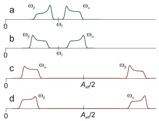
Figure 4.8: Solid-state nuclear frequency spectra for cases with negative nuclear Zeeman frequency . (a) Weak-coupling case with and . (b) Weak-coupling case with and . (a) Strong-coupling case with and . (b) Strong-coupling case with and .

14.5. Exchange interaction

14.5.1. Physical origin and consequences of the exchange interaction

If two unpaired electrons occupy SOMOs in the same molecule or in spatially close molecules, the wave functions and of the two SOMOs may overlap. The two unpaired electrons can couple either to a singlet state or to a triplet state. The energy difference between the singlet and triplet state is the exchange integral

There exist different conventions for the sign of and the factor 2 may be missing in parts of the literature. With the sign convention used here, the singlet state is lower in energy for positive . Since the singlet state with spin wave function is antisymmetric with respect to exchange of the two electrons and electrons are Fermions, it corresponds to the situation where the two electrons could also occupy the same orbital. This is a bonding orbital overlap, corresponding to an antiferromagnetic spin ordering. Negative correspond to a lower-lying triplet state, i.e., antibonding orbital overlap and ferromagnetic spin ordering. The triplet state has three substates with wave functions for the state, for the state, and for the state. The and state are eigenstates both in the absence and presence of the coupling. The states and are eigenstates for , where is the difference between the electron Zeeman frequencies of the two spins. For the opposite case of , the eigenstates are and . The latter case corresponds to the high-field approximation with respect to the exchange interaction.

For strong exchange, , the energies are approximately for the singlet state and and for the triplet substates , and , respectively, where is the electron Zeeman interaction, which is the same for both spins within this approximation. If , microwave photons with energy cannot excite transitions between the singlet and triplet subspace of spin Hilbert space. It is then convenient to use a coupled representation and consider the two subspaces separately from each other. The singlet subspace corresponds to a diamagnetic molecule and does not contribute to EPR spectra. The triplet subspace can be described by a group spin of the two unpaired electrons. In the coupled representation, does not enter the spin Hamiltonian, as it shifts all subspace levels by the same energy. For , the triplet state is the ground state and is always observable by EPR spectroscopy. However, usually one has and the singlet state is the ground state. As long as does not exceed thermal energy by a large factor, the triplet state is thermally excited and observable. In this case, EPR signal amplitude may increase rather than decrease with increasing temperature. For organic molecules, this case is also rare. If , the compound does not give an EPR signal. It may still be possible to observe the triplet state transiently after photoexcitation to an excited singlet state and intersystem crossing to the triplet state.

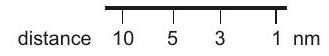
Weak exchange coupling is observed in biradicals with well localized SOMOs that are separated on length scales between and . In such cases, exchange coupling decreases exponentially with the distance between the two electrons or with the number of conjugated bonds that separate the two centers of spin density. If the two centers are not linked by a continuous chain of conjugated bonds, exchange coupling is rarely resolved at distances larger than . In any case, at such long distances exchange coupling is much smaller than the dipole-dipole coupling between the two unpaired electrons if the system is not conjugated. For weak exchange coupling, the system is more conveniently described in an uncoupled representation with two spins and .

Exchange coupling is also significant during diffusional encounters of two paramagnetic molecules in liquid solution. Such dynamic Heisenberg spin exchange can be pictured as physical exchange of unpaired electrons between the colliding molecules. This causes a sudden change of the spin Hamiltonian, which leads to spin relaxation. A typical example is line broadening in EPR spectra of radicals by oxygen, which has a paramagnetic triplet ground state. If radicals of the same type collide, line broadening is also observed, but the effects on the spectra can be more subtle, since the spin Hamiltonians of the colliding radicals are the same. In this case, exchange of unpaired electrons between the radicals changes only spin state, but not the spin Hamiltonian.

14.5.2. Exchange Hamiltonian

The spin Hamiltonian contribution by weak exchange coupling is

This Hamiltonian is analogous to the coupling Hamiltonian in NMR spectroscopy. If the two spins have different values and the field is sufficiently high , the exchange Hamiltonian can be truncated in the same way as the coupling Hamiltonian in heteronuclear NMR:

14.5.3. Spectral manifestation of the exchange interaction

In the absence of hyperfine coupling, the situation is the same as for coupling in NMR spectroscopy. Exchange coupling between like spins (same electron Zeeman frequency) does not influence the spectra. For radicals in liquid solution, hyperfine coupling is usually observable. In this case, exchange coupling does influence the spectra even for like spins, as illustrated in Figure for two exchange-coupled electron spins and with each of them coupled exclusively to only one nuclear spin and , respectively) with the same hyperfine coupling . If the exchange coupling is much smaller than the isotropic hyperfine coupling, each of the individual lines of the hyperfine triplet further splits into three lines. If the splitting is very small, it may be noticeable only as a line broadening. At very large exchange coupling, the electron spins are uniformly distributed over the two exchange-coupled moieties. Hence, each of them has the same hyperfine coupling to both nuclei. This coupling is half the original hyperfine coupling, since, on average, the electron spin has only half the spin density in the orbitals of a given nucleus as compared to the case without exchange coupling. For intermediate exchange couplings, complex splitting patterns arise that are characteristic for the ratio between the exchange and hyperfine coupling.

Figure 5.1: Influence of the exchange coupling on EPR spectra with hyperfine coupling in liquid solution (simulation). Spectra are shown for two electron spins and with the same isotropic value and the same isotropic hyperfine coupling to a nuclear spin or , respectively. In the absence of exchange coupling, a triplet with amplitude ratio is observed. For small exchange couplings, each line splits into a triplet. At intermediate exchange couplings, complicated patterns with many lines result. For very strong exchange coupling, each electron spin couples to both nitrogen nuclei with half the isotropic exchange coupling. A quintuplet with amplitude ratio is observed.

15. Dipole-dipole interaction

15.5.4. Physical picture

The magnetic dipole-dipole interaction between two localized electron spins with magnetic moments and takes the same form as the classical interaction between two magnetic point dipoles. The interaction energy

generally depends on the two angles and that the point dipoles include with the vector between them and on the dihedral angle (Figure 5.2). The dipole-dipole interaction scales with the inverse cube of the distance between the two point dipoles.

In general, the two electron spins are spatially distributed in their respective SOMOs. The point-dipole approximation is still a good approximation if the distance is much larger than the spatial distribution of each electron spin. Further simplification is possible if anisotropy is much smaller than the isotropic value. In that case, the two spins are aligned parallel to the magnetic field and thus also parallel to each other, so that and . Eq. (5.4) then simplifies to

which is the form known from NMR spectroscopy.

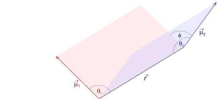
Figure 5.2: Geometry of two magnetic point dipoles in general orientation. Angles and are included between the respective magnetic moment vectors or and the distance vector between the point dipoles. Angle is the dihedral angle.

15.5.5. Dipole-dipole Hamiltonian

For two electron spins that are not necessarily aligned parallel to the external magnetic field, the dipole-dipole coupling term of the spin Hamiltonian assumes the form

If the electrons are distributed in space, the Hamiltonian has to be averaged (integrated) over the two spatial distributions, since electron motion proceeds on a much faster time scale than an EPR experiment.

If the two unpaired electrons are well localized on the length scale of their distances and their spins are aligned parallel to the external magnetic field, the dipole-dipole Hamiltonian takes the form

with the terms of the dipolar alphabet

Usually, EPR spectroscopy is performed at fields where the electron Zeeman interaction is much larger than the dipole-dipole coupling, which has a magnitude of about at a distance of and of at a distance of . In this situation, the terms , and are non-secular and can be dropped. The term is pseudo-secular and can be dropped only if

Figure 5.3: Explanation of dipole-dipole coupling between two spins in a local field picture. At the observer spin (blue) a local magnetic field is induced by the magnetic moment of the coupling partner spin (red). In the secular approximation only the component of this field is relevant, which is parallel or antiparallel to the external magnetic field . The magnitude of this component depends on angle between the external magnetic field and the spin-spin vector . For the (left) and (right) states of the partner spin, the local field at the observer spin has the same magnitude, but opposite direction. In the high-temperature approximation, both these states are equally populated. The shift of the resonance frequency of the observer spin thus leads to a splitting of the observer spin transition, which is twice the product of the local field with the gyromagnetic ratio of the observer spin.

the difference between the electron Zeeman frequencies is much larger than the dipole-dipole coupling 1 . In electron electron double resonance (ELDOR) experiments, the difference of the Larmor frequencies of the two coupled spins can be selected via the difference of the two microwave frequencies. It is thus possible to excite spin pairs for which only the secular part of the spin Hamiltonian needs to be considered,

with

The dipole-dipole coupling then has a simple dependence on the angle between the external magnetic field and the spin-spin vector and the coupling can be interpreted as the interaction of the spin with the component of the local magnetic field that is induced by the magnetic dipole moment of the coupling partner (Figure 5.3). Since the average of the second Legendre polynomial over all angles vanishes, the dipole-dipole interaction vanishes under fast isotropic motion. Measurements of this interaction are therefore performed in the solid state.

The dipole-dipole tensor in the secular approximation has the eigenvalues . The dipole-dipole coupling at any orientation is given by

15.5.6. Spectral manifestation of the dipole-dipole interaction

The energy level scheme and a schematic spectrum for a spin pair with fixed angle are shown in Figure and b, respectively. The dipole-dipole couplings splits the transition of either coupled spin by . If the sample is macroscopically isotropic, for instance a microcrystalline powder or a glassy frozen solution, all angles occur with probability . Each line of the dipolar doublet

Hyperfine coupling of the electron spins can modify this condition.

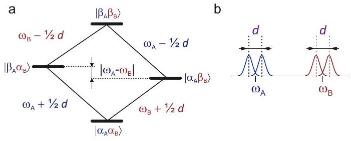
Figure 5.4: Energy level scheme (a) and schematic spectrum (b) for a dipole-dipole coupled spin pair at fixed orientation with respect to the magnetic field. The electron Zeeman frequencies of the two spins are and , respectively. Weak coupling is assumed. The dipolar splitting is the same for both spins. Depending on homogeneous linewidth , the splitting may or may not be resolved. If and are distributed, for instance by anisotropy, resolution is lost even for .

is then broadened to a powder pattern as illustrated in Figure 3.3. The powder pattern for the state of the partner spin is a mirror image of the one for the state, since the frequency shifts by the local magnetic field have opposite sign for the two states. The superposition of the two axial powder patterns is called Pake pattern (Figure 5.5). The center of the Pake pattern corresponds to the magic angle . The dipole-dipole coupling vanishes at this angle.

Figure 5.5: Pake pattern observed for a dipole-dipole coupled spin pair. (a) The splitting of the dipolar doublet varies with angle between the spin-spin vector and the static magnetic field. Orientations have a probability . (b) The sum of all doublets for a uniform distribution of directions of the spin-spin vector is the Pake pattern. The "horns" are split by and the "shoulders" are split by . The center of the pattern corresponds to the magic angle.

The Pake pattern is very rarely observed in an EPR spectrum, since usually other anisotropic interactions are larger than the dipole-dipole interaction between electron spins. If the weakcoupling condition is fulfilled for the vast majority of all orientations, the EPR lineshape is well approximated by a convolution of the Pake pattern with the lineshape in the absence of dipole-dipole interaction. If the latter lineshape is known, for instance from measuring analogous samples that carry only one of the two electron spins, the Pake pattern can be extracted by deconvolution and the distance between the two electron spins can be inferred from the splitting by inverting Eq. (5.15).

15.1. Zero-field interaction

15.1.1. Physical picture

If several unpaired spins are very strongly exchange coupled, then they are best described by a group spin . The concept is most easily grasped for the case of two electron spins that we have already discussed in Section 5.1.1. In this case, the singlet state with group spin is diamagnetic and thus not observable by EPR. The three sublevels of the observable triplet state with group spin correspond to magnetic quantum numbers , and at high field. These levels are split by the electron Zeeman interaction. The transitions and are allowed electron spin transitions, whereas the transition is a forbidden double-quantum transition.

At zero magnetic field, the electron Zeeman interaction vanishes, yet the three triplet sublevels are not degenerate, they exhibit zero-field splitting. This is because the unpaired electrons are also dipole-dipole coupled. Integration of Eq. (5.6) over the spatial distribution of the two electron spins in their respective SOMOs provides a zero-field interaction tensor that can be cast in a form where it describes coupling of the group spin with itself [Rie07]. At zero field, the triplet sublevels are not described by the magnetic quantum number , which is a good quantum number only if the electron Zeeman interaction is much larger than the zero-field interaction. Rather, the triplet sublevels at zero field are related to the principal axes directions of the zero-field interaction tensor and are therefore labeled , and , whereas the sublevels in the high-field approximation are labeled , and .

This concept can be extended to an arbitrary number of strongly coupled electron spins. Cases with up to 5 strongly coupled unpaired electrons occur for transition metal ions (d shell) and cases with up to 7 strongly coupled unpaired electrons occur for rare earth ions (f shell). According to Hund's rule, in the absence of a ligand field the state with largest group spin is the ground state. Kramers ions with an odd number of unpaired electrons have a half-integer group spin . They behave differently from non-Kramers ions with an even number of electrons and integer group spin . This classification relates to Kramers' theorem, which states that for a time-reversal symmetric system with half-integer total spin, all eigenstates occur as pairs (Kramers pairs) that are degenerate at zero magnetic field. As a consequence, for Kramers ions the ground state at zero field will split when a magnetic field is applied. For any microwave frequency there exists a magnetic field where the transition within the ground Kramers doublet is observable in an EPR spectrum. The same does not apply for integer group spin, where the ground state may not be degenerate at zero field. If the zero-field interaction is larger than the maximum available microwave frequency, non-Kramers ions may be unobservable by EPR spectroscopy although they exist in a paramagnetic high-spin state. Typical examples of such EPR silent non-Kramers ions are high-spin and high-spin . In rare cases, non-Kramers ions are EPR observable, since the ground state can be degenerate at zero magnetic field if the ligand field features axial symmetry. Note also that "EPR silent" non-Kramers ions can become observable at sufficiently high microwave frequency and magnetic field.

For transition metal and rare earth ions, zero-field interaction is not solely due to the dipole-dipole interaction between the electron spins. Spin-orbit coupling also contributes, in many cases even stronger than the dipole-dipole interaction. Quantum-chemical prediction of the zero-field interaction is an active field of research. Quite reasonable predictions can be obtained for transition metal ions, whereas only order-of-magnitude estimates are usually possible for rare earth ions.

15.1.2. Zero-field interaction Hamiltonian

The zero-field interaction Hamiltonian is often given as

where denotes the transpose of the spin vector operator. In the principal axes system of the zero-field splitting (ZFS) tensor, the Hamiltonian simplifies to

where and . The reduction to two parameters is possible, since is a traceless tensor. In other words, the zero-field interaction is purely anisotropic. The notation presumes that is the principal value with the largest absolute value can be negative). Together with the absence of an isotropic component, this means that , which is always the intermediate value, is either closer to than to or exactly in the middle between these two values. Accordingly, . At axial symmetry . Axial symmetry applies if the system has a symmetry axis with . At cubic symmetry, both and are zero. For group spin , the leading term of the is then a hexadecapolar contribution that scales with the fourth power of the spin operators .

In the high-field approximation the ZFS contribution to the Hamiltonian is a term. In other words, to first order in perturbation theory the contribution of the ZFS to the energy of a spin level with magnetic quantum number scales with . For an allowed transition , this contribution is . This contribution vanishes for the central transition of Kramers ions. More generally, because of the scaling of the level energies with to first-order, the contribution of ZFS to transition frequencies vanishes for all transitions.

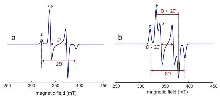
Figure 5.6: Schematic CW EPR spectra for triplet states at high field. Simulations were performed at an X-band frequency of . (a) Axial symmetry . The spectrum is the derivative of a Pake pattern. (b) Orthorhombic symmetry .

15.1.3. Spectral manifestation of zero-field splitting

Spectra are most easily understood in the high-field approximation. Quite often, deviations from this approximation are significant for the ZFS (see Fig. 2.2), and such deviations are discussed later. The other limiting case, where the ZFS is much larger than the electron Zeeman interaction (Fe(III) and most rare earth ions), is discussed in Section 5.3.4.

For triplet states with axial symmetry of the ZFS tensor, the absorption spectrum is a Pake pattern (see Section 5.2.3). With continuous-wave EPR, the derivative of the absorption spectrum is detected, which has the appearance shown in Fig. 5.6(a). A deviation from axial symmetry leads to a splitting of the "horns" of the Pake pattern by , whereas the "shoulders" of the pattern are not affected (Fig. 5.6(b)). Triplet states of organic molecules are often observed after optical excitation of a singlet state and intersystem crossing. Such intersystem crossing generally leads to different population of the zero-field triplet sublevels , and . In this situation the spin system is not at thermal equilibrium, but spin polarized. Such spin polarization affects relative intensity of the lineshape singularities in the spectra and even the sign of the signal may change. However, the singularities are still observed at the same resonance fields, i.e., the parameters and can still be read off the spectra as indicated in Fig. .

Even if the populations of the triple sublevels have relaxed to thermal equilibrium, the spectrum may still differ from the high-field approximation spectrum, as is illustrated in Fig. for the excited naphtalene triplet (simulation performed with an example script of the software package EasySpin http://WWW . easyspin.org/). For at a field of about (electron Zeeman frequency of about ) the high-field approximation is violated and is no longer a good quantum number. Hence, the formally forbidden double-quantum transition becomes partially allowed. To first order in perturbation theory, this transition is not broadened by the ZFS. Therefore it is very narrow compared to the allowed transitions and appears with higher amplitude.

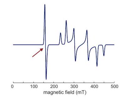
Figure 5.7: CW EPR spectrum of the excited naphtalene triplet at thermal equilibrium (simulation at an -band frequency of ). The red arrow marks the half-field signal, which corresponds to the formally forbidden double-quantum transition .

For Kramers ions, the spectra are usually dominated by the central transition, which is not ZFS-broadened to first order. To second order in perturbation theory, the ZFS-broadening of this line scales inversely with magnetic field. Hence, whereas systems with anisotropy exhibit broadening proportional to the magnetic field , central transitions of Kramers ions exhibit narrowing with . The latter systems can be detected with exceedingly high sensitivity at high fields if they do not feature significant anisotropy. This applies to systems with half-filled shells (e.g. ). In the case of Mn(II) (Figure 5.8) the narrow central transition is split into six lines by hyperfine coupling to the nuclear spin of (nuclear spin natural abundance). Because of the scaling of anisotropic ZFS broadening of transitions, satellite transitions become the broader the larger is for the involved levels. In the high-temperature approximation, the integral intensity in the absorption spectrum is the same for all transitions. Hence, broader transitions make a smaller contribution to the amplitude in the absorption spectrum and in its first derivative that is acquired by CW EPR.

Figure 5.8: CW EPR spectrum of a Mn(II) complex (simulation at a W-band frequency of ). . The six intense narrow lines are the hyperfine multiplet of the central transition .

The situation can be further complicated by and strain, which is a distribution of the and parameters due to a distribution in the ligand field. Such a case is demonstrated in Fig. for Gd(III) at a microwave frequency of where second-order broadening of the central transition is still rather strong. In such a case, lineshape singularities are washed out and ZFS parameters cannot be directly read off the spectra. In CW EPR, the satellite transitions may remain unobserved as the derivative of the absorption lineshape is very small except for the central transition.

15.1.4. Effective spin in Kramers doublets

For some systems, such as Fe(III), ZFS is much larger than the electron Zeeman interaction at any experimentally attainable magnetic field. In this case, the zero-field interaction determines the quantization direction and the electron Zeeman interaction can be treated as a perturbation [Cas+60]. The treatment is simplest for axial symmetry , where the quantization axis is the axis of the ZFS tensor. The energies in the absence of the magnetic field are

which for high-spin Fe(III) with gives three degenerate Kramers doublets corresponding to , and . If the magnetic field is applied along the axis of the ZFS tensor, is a good quantum number and there is simply an additional energy term with being the value for the half-filled shell, which can be approximated as . Furthermore, in this situation only the transition is allowed. The Zeeman term leads to a splitting of the Kramers doublet that is proportional to and

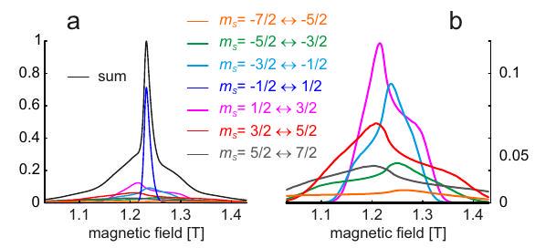
Figure 5.9: Echo-detected EPR spectrum (absorption spectrum) of a Gd(III) complex with GHz, a Gaussian distribution of with standard deviation of and a correlated distribution of (simulation at a Q-band frequency of courtesy of Dr. Maxim Yulikov). (a) Total spectrum (black) and contributions of the individual transitions (see legend). The signal from the central transition (blue) dominates. (b) Contributions of the satellite transitions scaled vertically for clarity.

corresponds to . This Kramers doublet can thus be described as an effective spin with .

If the magnetic field is perpendicular to the tensor axis, the and Kramers doublets are not split, since the and operator does not connect these levels. The operator has an off-diagonal element connecting the levels that is . Since the levels are degenerate in the absence of the electron Zeeman interaction, they become quantized along the magnetic field and is again a good quantum number of this Kramers doublet. The energies are , so that the transition frequency is again proportional to , but now with an effective value . Intermediate orientations can be described by assuming an effective tensor with axial symmetry and . This situation is encountered to a good approximation for high-spin Fe(III) in hemoglobins .

For the non-axial case , the magnetic field will split all three Kramers doublets. To first order in perturbation theory the splitting is proportional to , meaning that each Kramers doublet can be described by an effective spin with an effective tensor. Another simple case is encountered for extreme rhombicity, . By reordering principal axes (exchanging with either or ) one can the get rid of the term in Eq. (5.18), so that the ZFS Hamiltonian reduces to with . The level pair corresponding to the new direction of the tensor has zero energy at zero magnetic field and it can be shown that it has an isotropic effective value . Indeed, signals near are very often observed for high-spin Fe(III).

15.2. Physical picture

15.2.1. The spin system

The basic phenomena can be well understood in the simplest possible electron-nuclear spin system consisting of a single electron spin with isotropic value that is hyperfine coupled to a nuclear spin with a magnitude of the hyperfine coupling that is much smaller than the electron Zeeman interaction. In this situation the high-field approximation is valid for the electron spin, so that the hyperfine Hamiltonian can be truncated to the form given by Eq. (4.9). Because of the occurrence of an operator in this Hamiltonian, we cannot simply transform the Hamiltonian to the rotating frame for the nuclear spin . However, we don't need to, as we shall consider only microwave irradiation. For the electron spin , we transform to the rotating frame where this spin has a resonance offset . Hence, the total Hamiltonian takes the form

in the rotating frame for the electron spin and the laboratory frame for the nuclear spin. Such a Hamiltonian is a good approximation, for instance, for protons in organic radicals.

The Hamiltonian deviates from the Hamiltonian that would apply if the high-field approximation were also fulfilled for the nuclear spin. The difference is the pseudo-secular hyperfine coupling term . As can be seen from Eq. (4.10), this term vanishes if the hyperfine interaction is purely isotropic, i.e. for sufficiently fast tumbling in liquid solution, and along the principal axes of the hyperfine tensor. Otherwise, the term can only be neglected if , corresponding to the high-field approximation of the nuclear spin. Within the approximate range the pseudo-secular interaction may affect transition frequencies and makes formally forbidden transitions with partially allowed, as is no longer a good quantum number.

15.2.2. Local fields at the nuclear spin

The occurrence of forbidden transitions can be understood in a semi-classical magnetization vector picture by considering local fields at the nuclear spin for the two possible states and

The product of rotational correlation time and hyperfine anisotropy must be much smaller than unity

Figure 6.1: Local fields (multiplied by the gyromagnetic ratio of the nuclear spin) at the nuclear spin in the two states and of an electron spin . The quantization axes are along the effective fields and and are, thus, not parallel.

of the electron spin. These local fields are obtained from the parameters , and of the Hamilton operator terms that act on the nuclear spin. When divided by the gyromagnetic ratio of the nuclear spin these terms have the dimension of a local magnetic field. The local field corresponding to the nuclear Zeeman interaction equals the static magnetic field and is the same for both electron spin states, since the expectation value of does not depend on the electron spin state. It is aligned with the direction of the laboratory frame (blue arrow in Figure 6.1). Both hyperfine fields arise from Hamiltonian terms that contain an factor, which has the expectation value for the state and for the state. The term is aligned with the axis and directed towards in the state and towards in the state, assuming (violet arrows). The term is aligned with the axis and directed towards in the state and towards in the state, assuming (green arrows).

The effective fields at the nuclear spin in the two electron spins states are vector sums of the three local fields. Because of the component along , they are tilted from the direction by angle in the state and by angle in the state. The length of the sum vectors are the nuclear transition frequencies in these two states and are given by

For , the hyperfine splitting is given by

and the sum frequency is given by

For , the nuclear frequency doublet is centered at Fig. ). The sum frequency is always larger than twice the nuclear Zeeman frequency. None of the nuclear frequencies can become zero, the minimum possible value is attained in one of the electron spin states for matching of the nuclear Zeeman and hyperfine interaction at . For the nuclear frequency doublet is split by and centered at Fig. . The tilt angles and (Figure 6.1) can be inferred from trigonometric relations and are given by

Consider now a situation where the electron spin is in its state. The nuclear magnetization from all radicals in this state at thermal equilibrium is aligned with . Microwave excitation causes transitions to the state. In this state, the local field at the nuclear spin is directed along . Hence, the nuclear magnetization vector from the radicals under consideration is tilted by angle (Figure 6.1) with respect to the current local field. It will start to precess around this local field vector. This corresponds to excitation of the nuclear spin by flipping the electron spin, which is a formally forbidden transition. Obviously, such excitation will occur only if angle differs from and from . The case of corresponds to the absence of pseudo-secular hyperfine coupling and is also attained in the limit . The situation is attained in the limit of very strong secular hyperfine coupling, . Forbidden transitions are observed for intermediate hyperfine coupling. Maximum excitation of nuclear spins is expected when the two quantization axes are orthogonal with respect to each other, .

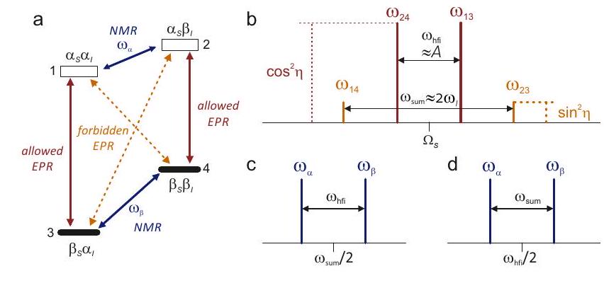
Figure 6.2: Electron-nuclear spin system in the presence of pseudo-secular hyperfine coupling. (a) Level scheme. In EPR, transitions are allowed (red), in NMR transitions are allowed (blue), and the zero- and double-quantum transitions with are formally forbidden. (b) EPR stick spectrum. Allowed transitions have transition probability and forbidden transitions probability . The spectrum is shown for . For , the forbidden transitions lie inside the allowed transition doublet. (c) NMR spectrum for . (d) NMR spectrum for .

15.3. Product operator formalism with pseudo-secular interactions

15.3.1. Transformation of to the eigenbasis

Excitation and detection in EPR experiments are described by the and operators in the rotating frame. These operators act only on electron spin transitions and thus formalize the spectroscopic selection rules. If the spin Hamiltonian contains off-diagonal terms, such as the pseudo-secular term in Eq. (6.1), the eigenbasis deviates from the basis of the electron spin rotating frame/nuclear spin laboratory frame in which the Hamiltonian is written and in which the excitation and detection operators are linear combinations of and . In order to understand which transitions are driven and detected with what transition moment, we need to transform to the eigenbasis (the transformation of is analogous). This can be done by product operator formalism and can be understood in the local field picture.

The Hamiltonian in the eigenbasis has no off-diagonal elements, meaning that all quantization axes are along . Thus, we can directly infer from Fig. that, in the state, we need a counterclockwise (mathematically positive) rotation by tilt angle about the axis, which is pointing into the paper plane. In the state, we need a clockwise (mathematically negative) rotation by tilt angle about the axis. The electron spin states can be selected by the projection operators and , respectively. Hence, we have to apply rotations and . These two rotations commute, as the and subspaces are distinct when is a good quantum number. For the rotation into the eigenbasis, we can write a unitary matrix

where and . Note that the definition of angle corresponds to the one given graphically in Fig. 6.1.2 The two new rotations about and also commute. Furthermore, commutes with and ), so that the transformation of to the eigenbasis reduces to

The transition moment for the allowed transitions that are driven by is multiplied by a factor , i.e. it becomes smaller when . In order to interpret the second term, it is best rewritten in terms of ladder operators and . We find

In other words, this term drives the forbidden electron-nuclear zero- and double-quantum transitions (Fig. 6.2(a)) with a transition proportional to .

In a CW EPR experiment, each transition must be both excited and detected. In other words, the amplitude is proportional to the square of the transition moment, which is the transition probability. Allowed transitions thus have an intensity proportional to and forbidden transitions a transition probability proportional to (Fig. 6.2(b)).

15.3.2. General product operator computations for a non-diagonal Hamiltonian

In a product operator computation, terms of the Hamiltonian can be applied one after the other if and only if they pairwise commute. This is not the case for the Hamiltonian in Eq. (6.1). However, application of diagonalizes the Hamiltonian:

This provides a simple recipe for product operator computations in the presence of the pseudosecular hyperfine coupling. Free evolution and transition-selective pulses are computed in the

We have used and . eigenbasis, using the Hamiltonian on the right-hand side of relation (6.9). For application of non-selective pulses, the density operator needs to be transformed to the electron spin rotating frame/nuclear spin laboratory frame basis by applying . In product operator formalism this corresponds to a product operator transformation . After application of non-selective pulses, the density operator needs to be backtransformed to the eigenbasis. Detection also needs to be performed in the electron spin rotating frame/nuclear spin laboratory frame basis.

This concept can be extended to any non-diagonal Hamiltonian as long as one can find a unitary transformation that transforms the Hamiltonian to its eigenbasis and can be expressed by a single product operator term or a sum of pairwise commuting product operator terms.

15.4. Generation and detection of nuclear coherence by electron spin excitation

15.4.1. Nuclear coherence generator

We have seen that a single microwave pulse can excite coherence on forbidden electron-nuclear zero- and double-quantum transitions. In principle, this provides access to the nuclear frequencies and , which are differences of frequencies of allowed and forbidden electron spin transitions, as can be inferred from Fig. 6.2(a,b). Indeed, the decay of an electron spin Hahn echo echo as a function of is modulated with frequencies and as well as with and ). Such modulation arises from forbidden transitions during the refocusing pulse, which redistribute coherence among the four transitions. The coherence transfer echoes are modulated by the difference of the resonance frequencies before and after the transfer by the pulse, in which the resonance offset cancels, while the nuclear spin contributions do not cancel. This two-pulse ESEEM experiment is not usually applied for measuring hyperfine couplings, as the appearance of the combination frequencies and complicates the spectra and linewidth is determined by electron spin transverse relaxation, which is much faster the nuclear spin transverse relaxation.

Better resolution and simpler spectra can be obtained by indirect observation of the evolution of nuclear coherence. Such coherence can be generated by first applying a pulse to the electron spins, which will generate electron spin coherence on allowed transitions with amplitude proportional to and on forbidden transitions with amplitude proportional to sin . After a delay a second pulse is applied. Note that the block is part of the EXSY and NOESY experiments in NMR. The second pulse will generate an electron spin magnetization component along for half of the existing electron spin coherence, i.e., it will "switch off" half the electron spin coherence and convert it to polarization. However, for the coherence on forbidden transitions, there is a chance that the nuclear spin is not flipped, i.e. that the coherent superposition of the nuclear spin states survives. For electron spin coherence on allowed transitions, there is a chance that the "switching off" of the electron coherence will lead to a "switching on" of nuclear coherences. Hence, in both these pathways there is a probability proportional to that nuclear coherence is generated. The delay is required, since at the different nuclear coherence components have opposite phase and cancel.

The nuclear coherence generated by the block can be computed by product operator formalism as outlined in Section 6.2.2. We find

This expression can be interpreted in the following way. Nuclear coherence is created with a phase as if it had started to evolve as at time (last cosine factors on the right-hand side of each line). It is modulated as a function of the electron spin resonance offset and zero exactly on resonance (first factor on each line). The integral over an inhomogeneously broadened, symmetric EPR line is also zero, since . However, this can be compensated later by applying another pulse. The amplitude of the nuclear coherence generally scales with , since one allowed and one forbidden transfer are required to excite it and (second factor). The third factor on the right-hand side of lines 1 and 2 tells that the amplitude of the coherence with frequency is modulated as a function of with frequency . Likewise, the amplitude of the coherence with frequency is modulated as a function of with frequency (lines 3 and 4 ). At certain values of no coherence is created at the transition with frequency , at other times maximum coherence is generated. Such behavior is called blind-spot behavior. In order to detect all nuclear frequencies, an experiment based on the nuclear coherence generator has to be repeated for different values of . Why and how CW EPR spectroscopy is done Sensitivity advantages of CW EPR spectroscopy The CW EPR experiment

Considerations on sample preparation Theoretical description of CW EPR Spin packet lineshape Saturation

16. 7 - CW EPR Spectroscopy

16.1. Why and how CW EPR spectroscopy is done

16.1.1. Sensitivity advantages of CW EPR spectroscopy

In NMR spectroscopy, CW techniques have been almost completely displaced by Fourier transform (FT) techniques, except for a few niche applications. FT techniques have a sensitivity advantage if the spectrum contains large sections of baseline and the whole spectrum can be excited simultaneously by the pulses. Neither condition is usually fulfilled in EPR spectroscopy. For two reasons, FT techniques lose sensitivity in EPR spectroscopy compared to the CW experiment. First, while typical NMR spectra comfortably fit into the bandwidth of a welldesigned critically coupled radiofrequency resonance circuit, EPR spectra are much broader than the bandwidth of a microwave resonator with high quality factor. Broadening detection bandwidth and proportionally lowering the quality factor of the resonator reduces signal-to-noise ratio unless the absorption lineshape is infinitely broad. A quality factor of the order of 10 ' 000 , which can be achieved with cavity resonators, corresponds to a bandwidth of roughly at X-band frequencies around . The intrinsic high sensitivity of detection in such a narrow band can be used only in a CW experiment. Second, even if the resonator is overcoupled to a much lower quality factor or resonators with intrinsically lower are used (the sensitivity loss can partially be compensated by a higher filling factor of such resonators), residual power from a high-power microwave pulse requires about in order to decay below the level of an EPR signal. This dead time is often a significant fraction of the transverse relaxation time of electron spins, which entails signal loss by relaxation. In contrast, in NMR spectroscopy the dead time is usually negligibly short compared to relaxation times. In many cases, the dead time in pulsed EPR spectroscopy even strongly exceeds . In this situation FT EPR is impossible, even with echo refocusing, while CW EPR spectra can still be measured. This case usually applies to transition metal complexes at room temperature and to many rare earth metal complexes and high-spin Fe(III) complexes even down to the boiling point of liquid helium at normal pressure (4.2 K). For these reasons, any unknown potentially paramagnetic sample should first be characterized by CW EPR spectroscopy. Pulsed EPR techniques are required if the resolution of CW EPR spectroscopy provides insufficient information to assign a structure. This applies mainly to small hyperfine couplings in organic radicals and of ligand nuclei in transition metal complexes (see Chapter 8) and to the measurement of distances between electron spins in the nanometer range (see Chapter 9). At temperatures where pulse EPR signals can be obtained, measurement of relaxation times is also easier and more precise with pulsed EPR techniques.

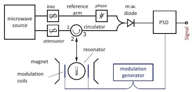
Figure 7.1: Scheme of a CW EPR spectrometer. Microwave from a fixed-frequency source is passed through an attenuator for adjusting its power and then through a circulator to the sample. Microwave that comes back from the sample passes on a different way through the same circulator and is combined with reference microwave of adjustable power (bias) and phase before it is detected by a microwave diode. The output signal of this diode enters a phase-sensitive detector (PSD) where it is demodulated with respect to the field modulation frequency (typically ) and at the same time amplified. The output signal of the PSD is digitized and further processed in a computer. The spectrum is obtained by sweeping the static magnetic field at constant microwave frequency.

16.1.2. The CW EPR experiment

Since the bandwidth of an optimized microwave resonator is much smaller than the typical width of EPR spectra, it is impractical to sweep the frequency at constant magnetic field in order to obtain a spectrum. Instead, the microwave frequency is kept constant and coincides with the resonator frequency at all times. The resonance condition for the spins is established by sweeping the magnetic field . Another difficulty arises from the weak magnetic coupling of the spins to the exciting electromagnetic field. Only a very small fraction of the excitation power is therefore observed. This problem is solved as follows. First, direct transmission of excitation power to the detector is prevented by a circulator (Figure 7.1). Power that enters port 1 can only leave to the sample through port 2 . Power that comes from the sample through port 2 can only leave to the detector diode through port 3. Second, the resonator is critically coupled. This means that all microwave power coming from the source that is incident to the resonator enters the resonator and is converted to heat by the impedance (complex resistance) of the resonator. If the sample is off resonant and thus does not absorb microwave, no microwave power leaves the resonator through port 3. If now the magnetic field is set to the resonance condition and the sample resonantly absorbs microwave, this means that the impedance of resonator + sample has changed. The resonator is no longer critically coupled and some of the incoming microwave is reflected. This microwave leaves the circulator through port 3 and is incident on the detector diode.

This reflected power at resonance absorption can be very weak at low sample concentration. It is therefore important to detect it sensitively. A microwave diode is only weakly sensitive to a change in incident power at low power (Fig. 7.2, input voltage is proportional to the square root of power). The diode is most sensitive to amplitude changes near its operating point, marked green in Fig. 7.2. Hence, the diode must be biased to its operating point by adding constant power from a reference arm. The phase of the reference arm must be adjusted so that microwave coming from the resonator and microwave coming from the reference arm interfere constructively.

Figure 7.2: Characteristic curve of a microwave detection diode. At small input voltage, the diode is rather insensitive to changes in input voltage. At the operating point (green), dependence of output current on input voltage is linear and has maximum slope. This corresponds to output current. If input voltage is too large, the diode is destroyed (red point).

A further problem arises from the fact that microwave diodes are broadband detectors. On the one hand, this is useful, since samples can significantly shift resonator frequency. On the other hand, broadband detectors also collect noise from a broad frequency band. This decreases signal-to-noise ratio and must be countered by limiting the detection bandwidth to the signal bandwidth or even below. Such bandwidth limitation can be realized most easily by effect modulation and phase sensitive detection. By applying a small sinusoidal magnetic field modulation with typical frequency of and typical amplitude of , the signal component at detector diode output becomes modulated with the same frequency, whereas noise is uncorrelated to the modulation. Demodulation with a reference signal from the field modulation generator (Figure 7.1) by a phase-sensitive detector amplifies the signal and limits bandwidth to the modulation frequency.

Effect modulation with phase-sensitive detection measures the derivative of the absorption lineshape, as long as the modulation amplitude is much smaller than the width of the EPR line (Fig. 7.3). Since signal-to-noise ratio is proportional to , one usually measures at , where lineshape distortion is tolerable for almost all applications. Precise lineshape analysis may require , whereas maximum sensitivity at the expense of significant artificial line broadening is obtained at . The modulation frequency should not be broader than the linewidth in frequency units. However, with the standard modulation frequency of that corresponds on a magnetic field scale to only at , this is rarely a problem.

16.1.3. Considerations on sample preparation

Since electron spins have a much larger magnetic moment than nuclear spins, electron-electron couplings lead to significant line broadening in concentrated solutions. Concentrations of paramagnetic centers should not usually exceed in order to avoid such broadening. For organic radicals in liquid solution it may be necessary to dilute the sample to in order to achieve ultimate resolution. For paramagnetic metal dopants in diamagnetic host compounds, at most of the diamagnetic sites should be substituted by paramagnetic centers. Such concentrations can be detected easily and with good signal-to-noise ratio. For most samples, good spectra can be obtained down to the range in solution and down to the 100 ppm dopant range in solids.

Line broadening in liquid solution can also arise from diffusional collision of paramagnetic

Figure 7.3: Detection of the derivative lineshape by field modulation. The situation is considered at the instantaneous field during a field sweep (vertical dashed line) that is slow compared to the field modulation frequency of . Modulation of the magnetic field with amplitude (blue) causes a modulation of the output signal (red) with the same frequency and an amplitude . Phase-sensitive detection measures this amplitude , which is proportional to the derivative of the grey absorption lineshape and to , as long as is much smaller than the peak-to-peak linewidth of the line. In practice, is usually acceptable. For precise lineshape analysis, is recommended.

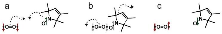
Figure 7.4: Relaxation enhancement by collisional exchange with oxygen in solution. (a) Situation before diffusional encounter. As an example, triplet oxygen is assumed to be in a state (red), whereas the spin of a nitroxide radical is assumed to be (green). (b) The oxygen molecule and nitroxide radical have collided during diffusional encounter. Their wavefunctions overlap and the three unpaired electrons cannot be distinguished from each other (grey). (c) After separation, the three unpaired electrons have been redistributed arbitrarily to the two molecules. For example, oxygen may now be in the state (red) and the nitroxide in the state (green). The electron spin of the nitroxide radical has flipped.

species with paramagnetic triplet oxygen (Figure 7.4). During such a collision, wavefunctions of the two molecules overlap and, since electrons are undistinguishable particles, spin states of all unpaired electrons in both molecules are arbitrarily redistributed when the two molecules separate again. The stochastic diffusional encounters thus lead to additional flips of the observed electron spins, which corresponds to relaxation and shortens longitudinal relaxation time . Since the linewidth is proportional to and cannot be longer than , frequent collisional encounters of paramagnetic species lead to line broadening. Such line broadening increases with decreasing viscosity (faster diffusion) and increasing oxygen concentration. The effect is stronger in apolar solvents, where oxygen solubility is higher than in polar solvents, but it is often significant even in aqueous solution. Best resolution is obtained if the sample is free of oxygen. The same mechanism leads to line broadening at high concentration of a paramagnetic species in liquid solution. In the solid state, line broadening at high concentration is mainly due to dipole-dipole coupling. Often, the anisotropically broadened EPR spectrum in the solid state is of interest, as it provides information on anisotropy and anisotropic hyperfine couplings. This may require freezing of a solution of the species of interest. Usually, the species will precipitate if the solvent crystallizes, which may cause line broadening and, in extreme cases, even collapse of the hyperfine structure and averaging of anisotropy by exchange between neighboring paramagnetic species. These problems are prevented if the solvent forms a glass, as is often the case for solvents that have methyl groups or can form hydrogen bonds in very different geometries. Typical glass-forming solvents are toluene, 2-methyltetrahydrofuran, ethanol, ethylene glycol, and glycerol. Aqueous solutions require addition of at least glycerol as a cryoprotectant. In most cases, crystallization will still occur on slow cooling. Samples are therefore shock frozen by immersion of the sample tube into liquid nitrogen. Glass tubes would break on direct immersion into liquid nitrogen, but EPR spectra have to be measured in fused silica sample tubes anyway, since glass invariably contains a detectable amount of paramagnetic iron impurities.

16.2. Theoretical description of CW EPR

This section overlaps with Section of the NMR lecture notes.

16.2.1. Spin packet lineshape

All spins in a sample that have the same resonance frequency form a spin packet. In the following we also assume that all spins of a spin packet have the same longitudinal and transverse relaxation times and , respectively. If the number of spins in the spin packet is sufficiently large, we can assign a magnetization vector to the spin packet. Dynamics of this magnetization vector with equilibrium magnetization during microwave irradiation is described by the Bloch equations in the rotating frame. In EPR spectroscopy, it is unusual to use the gyromagnetic ratio. Hence, we shall denote the resonance offset by

where is the microwave frequency in frequency units. The rotating-frame Bloch equations for the three components of the magnetization vector can then be written as

where is the microwave field amplitude in angular frequency units and is the mean value in the plane perpendicular to the static magnetic field. The apparent sign difference for the and terms arises from the different sense of spin precession for electron spins compared to nuclear spins with a positive gyromagnetic ratio.

If the spin packet is irradiated at constant microwave frequency, constant microwave power, and constant static magnetic field for a sufficiently long time (roughly ), the magnetization vector attains a steady state. Although the static field is swept in a CW EPR experiment, assuming a steady state is a good approximation, since the field sweep is usually slow compared to and . Faster sweeps correspond to the rapid scan regime that is not treated in this lecture course. In the steady state, the left-hand sides of the differential equations (7.2) for the magnetization vector components must all be zero,

This linear system of equations has the solution

where is not usually detected, is in phase with the exciting microwave irradiation and corresponds to the dispersion signal, and is out of phase with the exciting irradiation and corresponds to the absorption line. Unperturbed lineshapes are obtained in the linear regime, where the saturation parameter

fulfills . One can easily ascertain from Eq. (7.4) that in the linear regime increases linearly with increasing , which corresponds to proportionality of the signal to the square root of microwave power. is very close to the equilibrium magnetization. Within this regime, a decrease of in microwave attenuation, i.e., a power increase by , increases signal amplitude by a factor of 2 . Lineshape does not depend on in the linear regime. Therefore, it is good practice to measure at the highest microwave power that is still well within the linear regime, as this corresponds to maximum signal-to-noise ratio. For higher power the line is broadened.

Within the linear regime, takes the form of a Lorentzian absorption line

with linewidth in angular frequency units. The peak-to-peak linewidth of the first derivative of the absorption line is . Since EPR spectra are measured by sweeping magnetic field, we need to convert to magnetic field units,

The linewidth of a spin packet is called homogeneous linewidth. If is the same for all spin packets, this homogeneous linewidth is proportional to , a fact that needs to be taken into account in lineshape simulations for systems with large anisotropy. For most samples, additional line broadening arises from unresolved hyperfine couplings and, in the solid state, anisotropy. Therefore, cannot usually be obtained by applying Eq. (7.7) to the experimentally observed peak-to-peak linewidth.

16.2.2. Saturation

For microwave power larger than in the linear regime, the peak-to-peak linewidth increases by a factor . If a weak signal needs to be detected with maximum signal-to-noise ratio it is advantageous to increase power beyond the linear regime, but not necessarily to the maximum available level. For very strong irradiation, , the term 1 can be neglected in the denominator of Eqs. (7.4) for the magnetization vector components. The on-resonance amplitude of the absorption line is then given by

i.e., it is inversely proportional to . In this regime, the amplitude decreases with increasing power of the microwave irradiation.

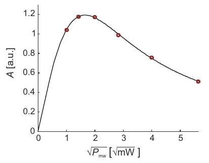
Figure 7.5: Progressive saturation measurement on the membrane protein LHCII solubilized in detergent micelles in nitrogen atmosphere. Residue V229 was mutated to cysteine and spin-labelled by iodoacetamidoPROXYL. Experimental data points (red) were obtained at microwave attenuations of , and with a full power of . The fit by Eq. (7.9) (black line) provides and .

Semi-quantitative information on spin relaxation can be obtained by the progressive power saturation experiment, where the EPR spectrum is measured as a function of microwave power . Usually, the peak-to-peak amplitude of the larges signal in the spectrum is plotted as a function of . Such saturation curves can be fitted by the equation

where the inhomogeneity parameter takes the value in the homogeneous limit and in the inhomogeneous limit. Usually, is not known beforehand and is treated as a fit parameter. The other fit parameters are , which is the slope of the amplitude increase with the square root of microwave power in the linear regime, and , which is the half-saturation power. More precisely, is the incident mw power where is reduced to half of its unsaturated value. Figure shows experimental data from a progressive saturation measurement on spin-labelled mutant V229C of major plant light harvesting complex LHCII solubilized in detergent micelles in a nitrogen atmosphere and a fit of this data by Eq. (7.9).

16.3. ENDOR

16.3.1. Advantages of electron-spin based detection of nuclear frequency spectra

Nuclear frequency spectra in the liquid (Section 4.3.2) and solid states (4.3.4) exhibit much better hyperfine resolution than EPR spectra, because the former spectra feature fewer and narrower lines. In fact, small hyperfine couplings to ligand nuclei in metal complexes are not usually resolved in EPR spectra and only the largest hyperfine couplings may be resolved in solid-state EPR spectra. The nuclear frequency spectra cannot be measured by a dedicated NMR spectrometer because they extend over several Megahertz to several tens of Megahertz, whereas NMR spectrometers are designed for excitation and detection bandwidths of a few tens of kilohertz. Furthermore, electron spin transitions have 660 times more polarization than proton transitions and more than that for other nuclei. Their larger magnetic moment also leads to higher detection sensitivity. It is thus advantageous to transfer polarization from electron spins to nuclear spins and to backtransfer the response of the nuclear spins to the electron spins for detection. Two classes of experiments can achieve this, electron nuclear double resonance (ENDOR) experiments, discussed in Section and electron spin echo envelope modulation (ESEEM) experiments discussed in Section 8.2.

16.3.2. Types of ENDOR experiments

An ENDOR experiment can be performed with strong CW irradiation of both electron and nuclear spins. In this CW ENDOR experiment, an electron spin transition is partially saturated, in Eq. (7.5). By driving a nuclear spin transition that shares an energy level with the saturated transition, additional relaxation pathways are opened up. The electron spin transition under observation is thus partially desaturated, and an increase in the EPR signal is observed. The experiment is performed at constant magnetic field with strong microwave irradiation at a maximum of the first-derivative absorption spectrum (i.e. the CW EPR spectrum) and the EPR signal is recorded as a function of the frequency of additional radiofrequency irradiation, which must fulfill the saturation condition for the nuclear spins. Usually, the radiofrequency irradiation is frequency modulated and the response is detected with another phase-sensitive detector, which leads to observation of the first derivative of the nuclear frequency spectrum. The CW ENDOR experiment depends critically on a balance of relaxation times, so that in the solid state sufficient sensitivity may only be achieved in a certain temperature range. Furthermore, simultaneous strong continuous irradiation by both microwave and radiofrequency, while keeping resonator frequency and temperature constant, is experimentally challenging. Therefore, CW ENDOR has been largely replaced by pulsed ENDOR techniques. However, for liquid solution samples CW ENDOR is usually the only applicable ENDOR technique.

The conceptually simplest pulsed ENDOR experiment is Davies ENDOR (Section 8.1.3), where saturation of the EPR transition is replaced by inversion by a pulse (Fig. 8.1(a)). A subsequent radiofrequency pulse, which is on-resonant with a transition that shares a level with the inverted EPR transition, changes population of this level and thus polarization of the EPR observer transition. This polarization change as a function of the radiofrequency is observed by a Hahn echo experiment on the observer transition. The approach works well for moderately large hyperfine couplings , in particular for nuclei directly coordinated to a transition metal ion or for protons at hydrogen-bonding distance or distances up to about Å. As we shall see in Section 8.1.3, the experiment is rather insensitive for very small hyperfine couplings.

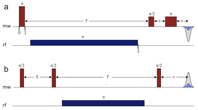
Figure 8.1: Pulsed ENDOR sequences. (a) Davies ENDOR. A selective inversion pulse on the electron spins is followed by a delay and Hahn echo detection (red). During microwave interpulse delay , a frequency-variable radiofrequency pulse is applied (blue). If this pulse is on resonant with a nuclear transition, the inverted echo recovers (pale blue). (b) Mims ENDOR. An non-selective stimulated echo sequence with interpulse delays and is applied to the electron spins (red). During microwave interpulse delay , a frequency-variable radiofrequency pulse is applied (blue). If this pulse is on resonant with a nuclear transition, the stimulated echo is attenuated (pale blue).

The smallest hyperfine couplings can be detected with the Mims ENDOR experiment that is based on the stimulated echo sequence Fig. b) ). The preparation block creates a polarization grating of the functional form , where is the EPR absorption spectrum as a function of the resonance offset and is the delay between the two microwave pulses. A radiofrequency pulse with variable frequency is applied during time when the electron spin magnetization is aligned with the axis. If this pulse is on resonant with a nuclear transition that shares a level with the observer EPR transition, half of the polarization grating is shifted by the hyperfine splitting , as will also become apparent in Section 8.1.3. For with integer the polarization grating is destroyed by destructive interference. Since the stimulated echo is the free induction decay (FID) of this polarization grating, it is canceled by a radiofrequency pulse that is on resonant with a nuclear transition. It is apparent that the radiofrequency pulse has no effect for with integer , where the original and frequency-shifted gratings interfere constructively. Hence, the Mims ENDOR experiment features blind spots as a function of interpulse delay . These blind spots are not a serious problem for very small hyperfine couplings . Note however that the first blind spot corresponds to . Hence, long interpulse delays are required in order to detect very small hyperfine couplings, and this leads to strong echo attenuation by a factor due to electron spin transverse relaxation. It can be shown that maximum sensitivity for very small couplings is attained approximately at .

Figure 8.2: Polarization transfer in Davies ENDOR. (a) Level populations at thermal equilibrium, corresponding to green label 0 in Fig. 8.1(a). The electron transitions (red, pale red) are much more strongly polarized than the nuclear transitions (blue, pale blue). (b) Level populations after a selective mw inversion pulse on resonance with the transition (dark red), corresponding to green label 1 in Fig. 8.1(a). A state of two-spin order is generated, where the two electron spin transitions are polarized with opposite sign and the same is true for the two nuclear spin transitions. (c) Level populations after a selective rf inversion pulse on resonance with the transition (dark blue), corresponding to green label 2 in Fig. 8.1(a). The electron spin observer transition is no longer inverted, but only saturated.

16.3.3. Davies ENDOR

The Davies ENDOR experiment is most easily understood by looking at the polarization transfers. At thermal equilibrium the electron spin transitions (red and pale red) are much more strongly polarized than the nuclear spin transitions (Fig. 8.2(a)). Their frequencies differ by an effective hyperfine splitting to a nuclear spin that is color-coded blue. The first microwave pulse is transition-selective, i.e., it has an excitation bandwidth that is smaller than . Accordingly, it inverts only one of the two electron spin transitions. We assume that the transition (red) is inverted and the transition (pale red) is not inverted; the other case is analogous. Such transition-selective inversion leads to a state of two-spin order, where all individual transitions in the two-spin system are polarized. However, the two electron spin transitions are polarized with opposite sign and the two nuclear transitions are also polarized with opposite sign (Fig. 8.2(b)). Now a radiofrequency pulse is applied. If this pulse is not resonant with a nuclear transition, the state of two-spin order persists and the observer electron spin transition (red) is still inverted. The radiofrequency pulse is also transition-selective. We now assume that this pulse inverts the transition (blue); the other case is again analogous. After such a resonant radiofrequency pulse, the two nuclear transitions are polarized with equal sign and the two electron spin transitions are saturated with no polarization existing on them (Fig. 8.2(c)). After the radiofrequency pulse a microwave Hahn echo sequence is applied resonant with the observer transition (Fig. 8.1(a)). If the radiofrequency pulse was off resonant (situation as in Fig. 8.2(b)), an inverted echo is observed. If, on the other hand, the radiofrequency pulse was on resonant (situation as in Fig. 8.2(c)) no echo is observed. In practice, polarization transfers are not complete and a weak echo is still observed. However, an on-resonant radiofrequency pulse causes some recovery of the inverted echo. If the radiofrequency is varied, recovery of the inverted echo is observed at all frequencies where the radiofrequency pulse is resonant with a nuclear transition.

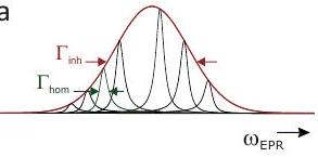
C

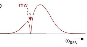
Figure 8.3: Spectral hole burning explanation of Davies ENDOR. (a) An inhomogeneously broadened EPR line with width (red) consists of many narrower homogeneously broadened lines with linewidth . (b) Long weak microwave irradiation saturates the on-resonant spin packet and does not significantly affect off-resonant spin packets. A spectral hole is burnt into the inhomogeneously broadened line, which can be as narrow as . (c) A selective microwave pulse burns an inversion hole into the EPR line whose width is approximately the inverse width of the pulse. (d) Situation after applying an on-resonant radiofrequency pulse. For the spin packet, where the microwave pulse was on-resonant with the transition, half of the spectral hole is shifted by to lower EPR frequencies. For the spin packet where the microwave pulse was on-resonant with the transition, half of the spectral hole is shifted by to higher EPR frequencies. Considering both cases, half of the hole persists, corresponding to saturation. Two side holes with a quarter of the depth of the inversion hole are created at . These side holes do not contribute to the echo signal, as long as they are outside the detection window (pale red) whose width is determined by the excitation bandwidth of the Hahn echo detection sequence.

Further understanding of Davies ENDOR is gained by considering an inhomogeneously broadened EPR line (Fig. 8.3). In such a line with width , each individual spin packet with much narrower width can, in principle, be selectively excited. A long rectangular pulse inverts the on-resonant spin packet and partially inverts spin packets roughly over a bandwidth corresponding to the inverse length of the pulse. In Davies ENDOR, pulse lengths between 50 and , corresponding to excitation bandwidths between 20 and are typical. Such a pulse creates an inversion hole centered at the microwave frequency . In an electron-nuclear spin system, two on-resonant spin packets exist, those where is the frequency of the transition and those where it is the frequency of the transition. For the former spin packet, inversion of the nuclear spin from the to the state increases the EPR frequency by the effective hyperfine splitting , whereas for the latter packet, inversion from the to the state decreases it by . In both cases half of the inversion hole is shifted to a side hole, leaving a saturation hole at and creating a saturation side hole. The saturation center holes of the two spin packets coincide in frequency and combine to a saturation hole in the inhomogeneously broadened line. At the side hole frequencies , only one of the two spin packets contributes to the hole, so that the side holes are only half as deep. The Hahn echo subsequence in the Davies ENDOR sequence must have a detection bandwidth that covers only the central hole (pale red in Fig. ), since no ENDOR effect would be observed if the side hole would also be covered. For this purpose, the detection bandwidth of the Hahn echo sequence can be limited either by using sufficiently long microwave pulses or by using a sufficiently long integration gate for the inverted echo.

In any case, a Davies ENDOR effect is only be observed if exceeds the width of the original inversion hole. The smaller , the longer the first inversion pulse needs to be and the fewer spin packets contribute to the signal. In general, hyperfine splittings much smaller than the homogeneous linewidth in the EPR spectrum cannot be detected. In practice, Davies ENDOR becomes very insensitive for pulse lengths exceeding 400 ns. If broadening of the inversion hole by electron spin relaxation is negligible, the suppression of signals with small hyperfine couplings in Davies ENDOR can be described by a selectivity parameter

where the length of the first mw pulse. Maximum absolute ENDOR intensity is obtained for . As a function of , the absolute ENDOR intensity is given by

The hyperfine contrast selectivity described by Eq. (8.2) can be used for spectral editing. For instance, ENDOR signals of directly coordinated ligand nitrogen atoms in transition metal complexes with of the order of overlap with ENDOR signals of weakly coupled ligand protons at X-band frequencies. At an inversion pulse length of about ENDOR signals are largely suppressed.

The sensitivity advantage of Mims ENDOR for very small hyperfine couplings can also be understood in the hole burning picture. Instead of a single center hole, a preparation block with nonselective microwave pulses creates a polarization grating that can be imagined as a comb of many holes that are spaced by frequency difference . The width of each hole is approximately . The width of the comb of holes is determined by the inverse length of the non-selective pulses, which are typically long. For small couplings, where in Davies ENDOR needs to be very long, more than an order of magnitude more spin packets take part in a Mims ENDOR experiment than in a Davies ENDOR experiment. The Mims ENDOR effect arises from the shift of one quarter of the polarization grating by frequency difference and one quarter of the grating by . The shifted gratings interfer with the grating at the center frequency. Depending on and on the periodicity of the grating, this interference is destructive (ENDOR effect) or constructive (no ENDOR effect).

16.4. ESEEM and HYSCORE

16.4.1. ENDOR or ESEEM?

In ESEEM experiments, polarization transfer from electron spins to nuclear spins and detection of nuclear frequencies on electron spin transitions are based on the forbidden electron-nuclear transitions discussed in Chapter 6. Much of the higher polarization of the electron spin transitions is lost in such experiments, since the angle between the quantization axes of the nuclear spin in the two electron spin states is usually small and the depth of nuclear echo modulations is sin . Furthermore, modulations vanish along the principal axes of the hyperfine tensor, where and thus . Therefore, lineshape singularities are missing in one-dimensional ESEEM spectra, which significantly complicates lineshape analysis. For this reason, one-dimensional ESEEM experiments are not usually competitive with ENDOR experiments, at least if the ENDOR experiments can be performed at -band frequencies or even higher frequencies. An exception arises for weakly coupled "remote" nuclei in transition metal complexes where exact cancellation between the nuclear Zeeman and the hyperfine interactions can be achieved for one of the electron spin states at X-band frequencies or slightly below. In this situation, pure nuclear quadrupole frequencies are observed, which leads to narrow lines and easily interpretable spectra. One-dimensional ESEEM data are also useful for determining local proton or deuterium concentrations around a spin label, which can be used as a proxy for water accessibility (Section 10.1.6).

The main advantage of ESEEM compared to ENDOR spectroscopy is the easier extension of ESEEM to a two-dimensional correlation experiment. Hyperfine sublevel correlation (HYSCORE) spectroscopy 8.2.3 resolves overlapping signal from different elements, simplifies peak assignment, and allows for direct determination of hyperfine tensor anisotropy even if the lineshape singularities are not observed.

16.4.2. Three-pulse ESEEM

The HYSCORE experiment is a two-dimensional extension of the three-pulse ESEEM experiment that we will treat first. In this experiment, the amplitude of a stimulated echo after is observed with the pulse sequence as a function of the variable interpulse delay at fixed interpulse delay (Fig. 8.4). The block serves as a nuclear coherence generator, as discussed in Section 6.3.1 and, simultaneously, creates the polarization grating discussed in the context of the Mims ENDOR experiment (Section 8.1.2). In fact, most of the thermal equilibrium magnetization is converted to the polarization grating whose FID after the final pulse is the stimulated echo, while only a small fraction is transferred to nuclear coherence. The phase of the nuclear coherence determines how much of it contributes to the stimulated echo after back transfer to electron spin coherence by the last pulse. For an electron-nuclear spin system this phase evolves with frequencies or if during interpulse delay the electron spin is in its or state, respectively. Hence, the part of the stimulated echo that arises from back transferred nuclear coherence is modulated as a function of with frequencies and .

An expression for the echo envelope modulation can be derived by product operator formalism using the concepts explained in Section 6.2. Disregarding relaxation, the somewhat lengthy derivation provides

where the terms and correspond to contributions with the electron spin in its or state, respectively, during interpulse delay . These terms are given by

The factors for the term and for the term describe the blind spot behavior of three-pulse ESEEM. The modulation depth is given by

For small hyperfine couplings, , we have , so that Eq. (8.5) reduces to

i.e., the modulation depth is inversely proportional to the square of the magnetic field. Using Eqs. (4.10) and (4.11) we find for protons not too close to a well localized unpaired electron

where is the angle between the electron-proton axis and the static magnetic field .

Because of the star topology of electron-nuclear spin systems (Fig. 4.4(a)), Eq. (8.3) can be easily extended by a product rule to multiple nuclei with spins , where is an index that runs over all nuclei. One finds

In the weak modulation limit, where all modulation depths fulfill the condition , the ESEEM spectrum due to several coupled nuclei is the sum of the spectra of the individual nuclei.

a

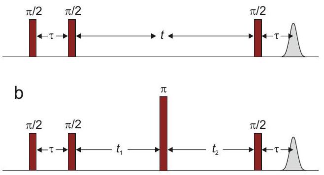
Figure 8.4: Pulse sequences for three-pulse ESEEM (a) and HYSCORE (b). In three-pulse ESEEM, time is varied and time is fixed. In HYSCORE, times and are varied independently in order to obtain a two-dimensional data set.

16.4.3. HYSCORE

The HYSCORE experiment is derived from the three-pulse ESEEM experiment by inserting a microwave pulse midway through the evolution of nuclear coherence. This splits the interpulse delay into two interpulse delays and (Fig. 8.4(b)), which are varied independently to provide a two-dimensional data set that depends parametrically on fixed interpulse delay . The inserted pulse inverts the electron spin state. Hence, coherence that has evolved with frequency during interpulse delay evolves with frequency during interpulse delay and vice versa. In the weak modulation limit, the HYSCORE experiment correlates only frequencies and of the same nuclear spin. The full modulation expression for the HYSCORE experiment contains a constant contribution and contributions that vary only with respect to either or . These contributions can be removed by background correction with low-order polynomial functions along both dimensions. The remaining modulation corresponds to only cross peaks and can be expressed as

with

In this representation with unsigned nuclear frequencies, one has for the weak coupling case and for the strong coupling case , as can be inferred from Fig. 6.1. Hence, in the weak coupling case and in the strong coupling case. In the weak coupling case, the cross peaks that correlate nuclear frequencies with the same sign ( terms) are much stronger than those that correlate frequencies with opposite terms) whereas it is the other way around in the strong coupling case. Therefore, the two cases can be easily distinguished in HYSCORE spectra, since the cross peaks appear in different quadrants (Fig. 8.5). Furthermore, disregarding a small shift that arises from the pseudo-secular part of the hyperfine coupling (see below), the cross peaks of a given isotope with spin are situated on parallels to the anti-diagonal that corresponds to the nuclear Zeeman frequency . This frequency in turn can be computed from the nuclear value (or gyromagnetic ratio ) and the static magnetic field . Peak assignment for nuclei is thus straightforward. For nuclei with the peaks are further split by the nuclear quadrupole interaction. Unless this splitting is much smaller than both the hyperfine interaction and the nuclear Zeeman interaction , numerical simulations are required to assign the peaks and extract the hyperfine and nuclear quadrupole coupling.

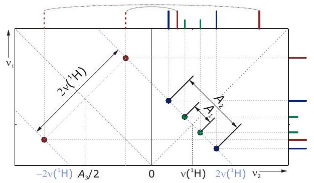
Figure 8.5: Schematic HYSCORE spectrum for the phenyl radical (compare Fig. 4.6). Note that hyperfine couplings are given here in frequency units, not angular frequency units. Signals from weakly coupled nuclei appear in the right quadrant. To first order, these peaks are situated on a line parallel to the anti-diagonal that intersects the axis at . The doublets are centered at and split by the respective hyperfine couplings. Signals from strongly coupled nuclei appear in the (-,+) quadrant. To first order, these peaks are situated on two lines parallel to the anti-diagonal that intersect the axis at and . The doublets are centered at half the hyperfine coupling and split by .

The small pseudo-secular shift of the correlation peaks with respect to the anti-diagonal contains information on the anisotropy of the hyperfine interaction (Fig. 8.5). In the solid state, the cross peaks from different orientations form curved ridges. For a hyperfine tensor with axial symmetry, as it is encountered for protons not too close to a well-localized unpaired electron, the maximum shift in the diagonal direction corresponds to and is given by . Since is known, , and thus the electron-proton distance can be computed from this maximum shift. If , which is usually the case, the orientation with maximum shift is at the same time the orientation with maximum modulation depth.

The curved ridges end at their intersection with the parallel to the anti-diagonal. These points correspond to the principal values of the hyperfine tensor and modulation depth is zero at these points. However, it is usually possible to fit the theoretical ridge to the experimentally observed ridge, as the curvature near together with the position of the point fully determines the problem.

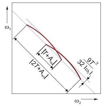
Figure 8.6: Schematic HYSCORE spectrum for a proton with an axial hyperfine tensor with anisotropy and isotropic component . The correlation peaks from different orientations form curved ridges (red). Curvature is the stronger the larger the anisotropy is and the ratio of squared anisotropy to the nuclear Zeeman frequency determines the maximum shift with respect to the anti-diagonal.

Analysis of HYSCORE spectra requires some precaution due to the blind-spot behavior (factor in Eq. (8.9)) and due to orientation selection by the limited bandwidth of the microwave pulses that is much smaller than spectral width for transition metal complexes. It is therefore prudent to measure HYSCORE spectra at several values of and at several observer positions within the EPR spectrum.

At a distance of between two localized unpaired electrons, splitting between the "horns" of the Pake pattern is about for two electron spins. Even strongly inhomogeneously broadened EPR spectra usually have features narrower than that (about in a magnetic field sweep). Depending on the width of the narrowest features in the EPR spectrum and on availability of an experimental spectrum or realistic simulated spectrum in the absence of dipole-dipole coupling, distances up to can be estimated from dipolar broadening by lineshape analysis. At distances below , such analysis becomes uncertain due to the contribution from exchange coupling between the two electron spins, which cannot be computed by first principles and cannot be predicted with sufficient accuracy by quantum-chemical computations. If the two unpaired electrons are linked by a continuous chain of conjugated bonds, exchange coupling can be significant up to much longer distances.

Distance measurements are most valuable for spin labels or native paramagnetic centers in biomolecules or synthetic macromolecules and supramolecular assemblies. In such systems, if the two unpaired electrons are not linked by a -electron system, exchange coupling is negligible with respect to dipole-dipole coupling for distances longer than . Such systems can often assume different molecular conformations, i.e. their structure is not perfectly defined. Structural characterization thus profits strongly from the possibility to measure distance distributions on length scales that are comparable to the dimension of these systems. This dimension is of the order of 2 to , corresponding to between and . In order to infer the distance distribution, this small dipole-dipole coupling needs to be separated from larger anisotropic interactions.

This separation of interactions is possible by observing the resonance frequency change for one spin in a pair (blue in Fig. 5.3) that is induced by flipping the spin of its coupling partner (red). In Fig. the resonance frequency of the observer spin before the flip of its coupling partner is indicated by a dashed line. If the coupling partner is in its state before the flip (left panel in Fig. 5.3), the local field at the observer spin will increase by upon flipping the coupling partner. This causes an increase of the resonance frequency of the observer spin by the dipole-dipole coupling (see Eq. (5.16)). If the coupling partner is in its state before the flip (right panel in Fig. 5.3), the local field at the observer spin will decrease by upon flipping the coupling partner. This causes an decrease of the resonance frequency of the observer spin by the dipole-dipole coupling . In the high-temperature approximation, both these cases have the

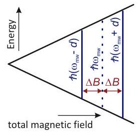
Figure 9.1: Resonance frequency shift of an observer spin (blue transitions) by the change in local magnetic field that arises upon a flip of a second spin that is dipole-dipole coupled to the observer spin. Compare Fig. for the local field picture.

same probability. Hence, half of the observer spins will experience a frequency change and the other half will experience a frequency change . If the observer spin evolves with changed frequency for some time , phases will be gained compared to the situation without flipping the coupling partner. The additional phase can be observed as a cosine modulation for both cases, as the cosine is an even function.

16.5. DEER

16.5.1. The four-pulse DEER experiment

The most commonly used experiment for distance distribution measurements in the nanometer range is the four-pulse double electron electron resonance (DEER) experiment (Figure 9.2), which is sometimes also referred to as pulsed electron electron double resonance (PELDOR) experiment. All interactions of the observer spin are refocused twice by two pulses at times and after the initial pulse. Repeated refocusing is necessary since all spin packets must be in phase at and overlap of the pump pulse with the observer pulse would lead to signal distortion. The first refocusing with interpulse delay restores the situation (1) immediately after the pulse with phase , where the magnetization vectors of all spin packets are aligned with the axis. In practice, coherence is excited on both observer spin transitions (blue in the energy level panels), but for clarity we consider only observer spin coherence that is on the upper transition and is symbolized by a wavy line in panel (1).

During time after the first refocusing, magnetization vectors of spin packets with different resonance offset dephase (panel (2)). Only the on-resonant spin packet, marked dark blue, is still aligned with the direction. The pump pulse flips the coupling partner and thus transfers the coherence to the lower observer spin transition. The resonance frequency of this transition is shifted by the dipole-dipole coupling in all spin packets. Observer spin magnetization further dephases until the time just before application of the second observer pulse (3)) and, in addition, the whole bundle of spin packet magnetization vectors precesses counterclockwise with the frequency shift . The originally on-resonant spin packet thus gains phase before the second observer pulse is applied. The second observer pulse with phase corresponds to a rotation about the axis. This mirrors the bundle of magnetization vectors with respect to the axis, inverting phase of the observer spin coherence (panel (4)). The bundle, which still

the first refocusing and all following magnetization panels are mirrored with respect to the axis.

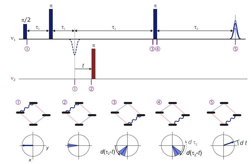
Figure 9.2: Four-pulse DEER sequence, coherence transfers, and evolution of the observer spin magnetization. Pulses shown in blue are applied to the observer spin, the pump pulse shown in red is applied to its coupling partner. The echo at time (dashed blue line) is not observed. Interpulse delays and are fixed, time is varied, and the echo amplitude is observed as a function of .

precesses counterclockwise with angular frequency now lags the axis by phase . During the final interpulse delay of length the bundle as a whole gains phase (grey arrow in panel (4) and simultaneously realigns along its center due to echo refocusing. However, the center corresponding to the originally on-resonant spin packet does not end up along , as it would have in the absence of the pump pulse. Rather, this spin packet has gained phase with respect to the direction (panel (5)). The magnetization vector component along , which corresponds to the echo signal, is given by .

The distance range of the DEER experiment is limited towards short distances by the requirement that, for echo refocusing, the observer pulses must excite both observer transitions, which are split by and, for coherence transfer, the pump pulse must excite both transitions of the coupling partner, which are also split by . In other words, both the observer refocused echo subsequence and the pump pulse must have an excitation bandwidth that exceeds . This requirement sets a lower distance bound of about at X-band frequencies and of about at -band frequencies. A limit towards long distances arises, since several dipolar oscillations need to be observed for inferring the width or even shape of a distance distribution and at least one oscillation needs to be observed for determining the mean distance. This requires . On the other hand, we have and the fixed interpulse delay cannot be much longer than the transverse relaxation time , since otherwise coherence has completely relaxed and no echos is observed. Electron spin transverse relaxation times are of the order of a few microseconds. Depending on sample type (see Section ), can be chosen between and , corresponding to maximum observable distances between 5 and .

16.5.2. Sample requirements

In the wanted coherence transfer pathway of the DEER experiment, observer pulses exclusively excite observer spins and the pump pulse exclusively excites the coupling partner. The excitation bandwidth must be sufficiently large to cover the dipole-dipole coupling at all orientations, i.e., larger than . If the two coupled spins have the same EPR spectrum, this spectrum must be broader than twice this minimum excitation bandwidth. This condition is fulfilled for nitroxide spin labels (Chapter 10) and transition metal ions at all EPR frequencies, whereas some organic radicals, such as trityl radicals, have spectra that are too narrow at X-band or even Q-band frequencies. Furthermore, must be sufficiently long for at least the observer spins. This condition can be fulfilled for almost all species at temperatures of (transition metal complexes) or (organic radicals), but may require cooling below for some high-spin species. For high-spin species with a half-filled valence shell, such as Mn(II) or measurement temperatures of are also sufficient.

Sample concentration should be sufficiently low for intermolecular distances to be much longer than intramolecular distances. For short distances, concentrations up to are possible, but concentrations of provide better results, if a spectrometer with sufficient sensitivity is available. Depending on distance and , measurements can be performed down to concentrations of . For membrane proteins reconstituted into liposomes, data quality is not only a function of bulk spin concentration, but also of lipid-to-protein ratio. This parameter needs to be optimized for each new protein. Required sample volume varies between a few microliters (W-band frequencies) and with at Q-band frequencies usually being optimal.

If concentration is not too high and the low-temperature limit of transverse relaxation can be attained, depends on the concentration and type of protons around the observer spin. Deuteration of the solvent and cryoprotectant (usually glycerol) usually dramatically improve data quality. If the matrix can be perdeuterated, deuteration of the protein or nuclei acid may further prolong and extend distance range or improve signal-to-noise ratio.

Complications arise if more than two unpaired electrons are found in the same molecule, but these complications can usually be solved. However, none of the spin pairs should have a distance shorter than the lower limit of the accessible distance range.

17. Conversion of dipolar evolution data to distance distributions

17.5.3. Expression for the DEER signal

In Section 9.1.1 we have seen that the echo is modulated with . Usually, this applies only to a fraction of the echo, because the pump pulse excites only a fraction of all spin packets of the coupling partner of the observer spin. Therefore, the echo signal for an isolated pair of electron spins in a fixed orientation with respect to the magnetic field is described by

where the dependence is given by Eqs. (5.16) and (5.15). The dependence cannot be expressed in closed form, but often is so weakly correlated with that it can be assumed as a constant, empirical parameter. In this situation, Eq. (9.1) can be integrated over all orientations

The pump pulse inverts not only the coupling partner of the observer spin in the same molecule, but also electron spins in remote other molecules. If these neighboring spins are homogeneously distributed in space, the background factor that arises from them assumes the form

where the orientation-averaged inversion efficiency is the fraction of spins excited by the pump pulse, is an average value, and is the total concentration of spins. For subtle reasons, differs significantly from the empirical two-spin modulation depth . Homogeneous distributions of neighboring spins that are nearly confined to a plane or a line give rise to a stretched exponential background function , where is a fractional dimension of the distribution that is usually somewhat larger than 2 or 1 for nearly planar or linear distributions, respectively. The total DEER signal is given by

If distance is distributed with normalized probability density , the form factor needs to be replaced by .

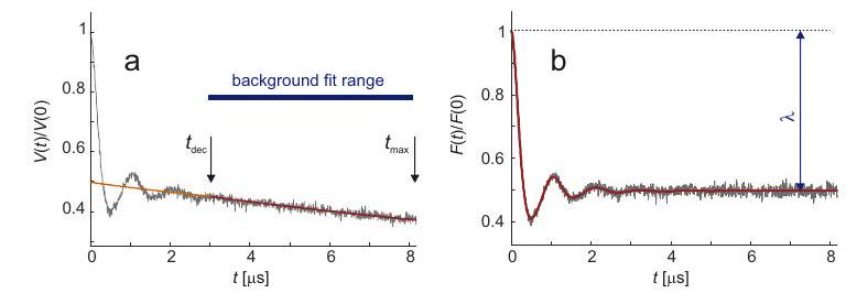
Figure 9.3: Background correction in DEER spectroscopy. (a) Primary data (simulation) normalized to . Dipolar modulation decays until a time . An exponentially decay function (red) is fitted to the data in the range , where is the maximum dipolar evolution time. This background function is extrapolated to the range (ochre). (b) The form factor is obtained by normalizing the background function, and dividing the normalized primary data by . It decays to a constant level , where is the modulation depth. The red curve is a simulation corresponding to the distance distribution extracted by Tikhonov regularization with optimum regularization parameter .

17.5.4. Background correction

The information on the distance distribution is contained in , which must thus be separated from . Often, the distribution is sufficiently broad for dipolar oscillations to decay within a time shorter than the maximum dipolar evolution time (Fig. 9.3(a)). For , the primary signal is then given by plus noise. The expression for is fitted to the primary data in this range (red line in Fig. 9.3(a)). In some cases, for instance for soluble proteins, a homogeneous distribution of molecules in three dimensions can be assumed, so that can be fixed. Otherwise, is treated as a fit parameter, as are and . The background function is obtained by extrapolating to the range (ochre line) and dividing it by . According to Eq. (9.4), the form factor results by dividing by . For narrow distance distributions, oscillations in may endure until the longest attainable . This does not create a problem if at least the first oscillation is completed well before . All the following oscillations have very similar amplitude and do not bias the background fit. As a rule of thumb, a good estimate for can be obtained by fitting data at if , i.e., if two full oscillations can be observed. If the data trace is shorter than that, background fitting is fraught with uncertainty. Wrong background correction may suppress long distances or create artificial peaks at long distances.

17.5.5. Tikhonov regularization with non-negativity constraint

In order to extract the distance distribution from the experimental form factor , we need to remove the constant contribution and renormalize to the dipolar evolution function

and invert the integral equation , where the kernel is given by

Here, we have substituted by by and reversed direction of the integration, which compensated for the negative in .

In practice, is digitized and given as a vector at sampling times . Likewise, it is sufficient to compute as a vector at sampling distances . The integral equation is thus transformed to a matrix equation

Unfortunately, this matrix equation cannot easily be inverted, since the rows of kernel are not orthogonal, i.e., the scalar product of dipolar evolution function vectors at different is not zero. The weak linear dependence of the rows makes the problem ill-posed. Small deviations of the experimental from the "true" , for instance due to noise, cause large deviations of from the true distance distribution. This problem can be solved only by taking into account additional information.

First, we know that, as a probability density, at all . Hence, we can impose a non-negativity constraint on . It turns out that this is not sufficient for stabilizing the solution. Noise can be fitted by ragged distance distributions with many narrow peaks, although we know that the distance distribution must be smooth, as it arises from a continuous distribution of molecular conformations. Tikhonov regularization imposes a smoothness restraint by minimizing

where

is the mean square deviation between experimental and simulated data and

is the square norm of the second derivative, which can be computed from by multiplication with the second derivative operator . The regularization parameter determines the relative

Figure 9.4: Tikhonov regularization of the data shown in Fig. 9.3. (a) L curve. The optimum regularization parameter corresponds to the corner (green circle) and provides the simulation shown in Fig. 9.3(b) as well as the extracted distance distribution shown as a black line in panel (c) of the current Figure. The red circle marks a too large regularization parameter that leads to oversmoothing. (b) Input form factor (black) and simulation for the too large regularization parameter corresponding to the red circle in the curve. (c) Theoretical distance distribution used for simulating a noiseless form factor (green) and distance distribution extracted from the noisy form factor with optimum regularization parameter corresponding to the green circle in the curve (black). (d) (c) Theoretical distance distribution used for simulating a noiseless form factor (green) and distance distribution extracted from the noisy form factor with a too large regularization parameter corresponding to the red circle in the curve (black).

weight of the smoothing restraint with respect to mean square deviation between experimental and simulated data. A parametric plot of versus as a function of is approximately L-shaped (Fig. 9.4). For very small , roughness of the distance distribution can be decreased strongly without increasing mean square deviation very much. For large is already smooth and a further increase of will lead only to a small decrease in roughness , but to a large increase in , since the overly broadened distance distribution no longer fits the dipolar oscillations. Hence, in a mathematical sense, the optimum regularization parameter corresponds to the corner of the curve. At this regularization parameter the extracted distance distribution (black line in Fig. 9.4(c)) is only slightly broader than the true distance distribution (green line) and the simulated form factor (red line in Fig. 9.3(b)) agrees with the experimental form factor (black line), except for the white noise contribution. If the regularization parameter is too large (red circle in Fig. 9.4(a)), the simulated form factor is overdamped (red line in Fig. 9.4(b)) and the distance distribution unrealistically broad (black line in Fig. 9.4(d)). For a too small regularization parameter the distance distribution unrealistically splits into several narrow peaks and the simulated form factor fits part of the noise (not shown). This error cannot be as clearly discerned in the simulated form factor as overdamping can be discerned. Undersmoothing is apparent only in the L curve.

Nitroxide spin probes and labels Spin probes and labels

Nitroxide radicals

The nitroxide EPR spectrum Influence of dynamics on the nitroxide spectrum Polarity and proticity

Water accessibility

Oxygen accessibility Local pH measurements

Spin traps

18. 0 - Spin Probes and Spin Traps

18.1. Nitroxide spin probes and labels

18.1.1. Spin probes and labels

Spin probes are stable paramagnetic species that are admixed to a sample in order to obtain structural or dynamical information on their environment and, thus, indirectly on the sample. Spin labels are spin probes that are covalently attached to a molecule of interest, often at a specific site. As compared to more direct characterization of structure and dynamics by other techniques, EPR spectroscopy on spin probes may be able to access other length and time scales or may be applicable in aggregation states or environments where these other techniques exhibit low resolution or do not yield any signal. Site-directed spin labeling (SDSL) has the advantage that assignment of the signal to primary molecular structure is already known and that a specific site in a complex system can be studied without disturbance from signals of other parts of the system. This approach profits from the rarity of paramagnetic centers. For instance, many proteins and most nucleic acids and lipids are diamagnetic. If a spin label is introduced at a selected site, EPR information is specific to this particular site.

In principle, any stable paramagnetic species can serve as a spin probe. Some paramagnetic metal ions can substitute for diamagnetic ions native to the system under study, as they have similar charge and ionic radius or with similar complexation properties as the native ions. This applies to , which can often substitute for without affecting function of proteins or nucleic acids, or Ln(III) lanthanide ions, which bind to Ca(II) sites. Paramagnetic metal ions can also be attached to proteins by engineering binding sites with coordinating amino acids, such as histidine, or by site-directed attachment of a metal ligand to the biomolecule. Such approaches are used for lanthanide ions, in particular Gd(III), and Cu(II).

For many spin probe approaches, organic radicals are better suited than metal ions, since in radicals the unpaired electron has closer contact to its environment (ligands screen environmental access of metal ions, in particular for lanthanide ions) and the EPR spectra are narrower, which allows for some experiments that cannot be performed on species with very broad spectra. Among organic radicals, nitroxides are the most versatile class of spin probes, mainly because of their relatively small size, comparable to an amino acid side group or nucleobase, and because of hyperfine and tensor anisotropy of a magnitude that is convenient for studying dynamics (Section 10.1.4). Triarylmethyl (TAM) radicals are chemically even more inert than nitroxide radicals and have slower relaxation times in liquid solution. Currently they are much less in use than nitroxide radicals, mainly because they are not commercially available and much harder to synthesize than nitroxide radicals.

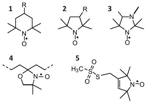
Figure 10.1: Structures of nitroxide probes. TEMPO derivatives. PROXYL derivatives. pH-sensitive imidazolidine nitroxide. 4 DOXYL derivatives. 5 Methanethiosulfonate spin label (MTSL)

18.1.2. Nitroxide radicals

The nitroxide radical is defined by the group, which is isoelectronic with the carbonyl group and can thus be replaced in approximate force field and molecular dynamics computations by a group. The unpaired electron is distributed over both atoms, which contributes to radical stability, with a slight preference for the oxygen atom. Nitroxide radicals become stable on the time scale of months or years if both positions are sterically protected, for instance by attaching two methyl groups to each of the atoms (Fig. 10.1). Nitroxides of this type are thermally stable up to temperatures of about , but they are easily reduced to the corresponding hydroxylamines, for instance by ascorbic acid, and are unstable at very low and very high pH. Nitroxides with five-membered rings (structures , and ) tend to be chemically more stable than those with six-membered rings (6). The five-membered rings also have less conformational freedom than the six-membered rings.

Spin probes can be addressed to certain environments in heterogeneous systems by choice of appropriate substituents (Fig. 10.1). The unsubstituted species are hydrophobic and partition preferably to nonpolar environments. Preference for hydrogen bond acceptors is achieved by hydroxyl derivatives , whereas ionic environments can be addressed by a carboxylate group at sufficiently high or by a trimethyl ammonium group . Reactive groups are used for SDSL, such as the methanethiosulfonate group in the dehydro-PROXYL derivative MTSL 5 , which selectively reacts with thiol groups under mild conditions. Thiol groups can be introduced into proteins by site-directed point mutation of an amino acid to cysteine and to RNA by replacement of a nucleobase by thiouridine. In DOXYL derivatives , a six-membered ring is spiro-linked to an alkyl chain, which can be part of stearic acid or of lipid molecules. The group in DOXYL derivatives is rigidly attached to the alkyl chain and nearly parallel to the axis of a hypothetical all-trans chain.

18.1.3. The nitroxide EPR spectrum

To a good approximation, the spin system of a nitroxide radical can be considered as an electron spin coupled to the nuclear spin of the atom of the group. Hyperfine

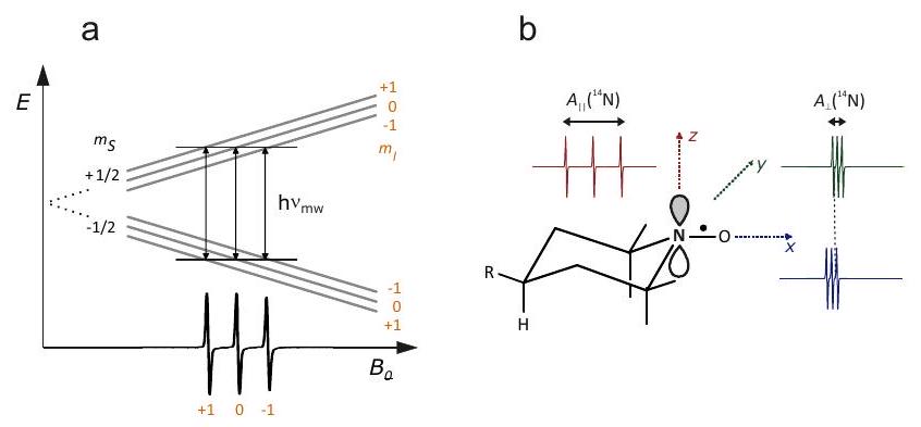
Figure 10.2: The EPR spectrum and molecular frame of nitroxide radicals. (a) The hyperfine sublevels corresponding to the three possible magnetic quantum numbers are shifted by . Allowed transitions are those with and . The microwave quantum has constant energy, since the microwave frequency is constant. During a magnetic field sweep, resonance is observed when the energy matches the energy difference of the levels of an allowed transition. The three transitions correspond to the three possible magnetic quantum numbers . (b) In a solid, each orientation gives a three-line spectrum, but the splitting and the center field depend on orientation, since and are anisotropic. To a good approximation, the hyperfine tensor has axial symmetry with the unique axis corresponding to the direction of the orbital lobes on the atom. The tensor is orthorhombic, i.e., the spectra in the plane of the molecular frame, which all have the same hyperfine splitting, have different center fields. The bond direction, which corresponds to the maximum value, is the molecular frame axis.

couplings to other nuclei, such as the methyl protons, are not usually resolved and contribute only to line broadening. The hyperfine coupling to the hybridized atom has a significant isotropic Fermi contact contribution from spin density in the orbital and a significant anisotropic contribution from spin density in the orbital that combines with a orbital on the oxygen atom to give the N-O bond partial double bond character. The direction of the lobes of the orbital is chosen as the molecular axis (Fig. 10.2(b)). The hyperfine tensor has nearly axial symmetry with being the unique axis. The hyperfine coupling is much larger along (on the order of ) than in the plane (on the order of ).

The spin-orbit coupling, which induces anisotropy, arises mainly at the atom, where a lone pair energy level is very close to the SOMO. The tensor is orthorhombic with nearly maximal asymmetry. The largest shift is positive and observed along the N-O bond, which is the molecular frame axis . An intermediate shift is observed along the axis , whereas the value is very close to . At X-band frequencies, where anisotropy corresponds to only dispersion in resonance fields, while hyperfine anisotropy corresponds to dispersion. At W-band frequencies, where , hyperfine anisotropy is still the same but anisotropy contributes a ten times larger dispersion of , which now dominates.

The field-swept CW EPR spectrum for a single orientation can be understood by considering the selection rule that the magnetic quantum number of the electron spin must change by 1 , whereas the magnetic quantum number of the nuclear spin must not change. Each transition can thus be assigned to a value of . For there are three such values, , and 1 (Fig. ). The microwave frequency is fixed and resonance is observed at fields where the energy of the microwave quantum matches the energy of a transition.

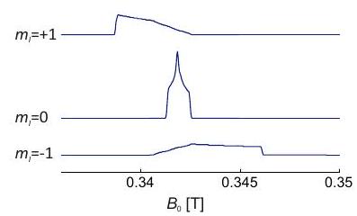
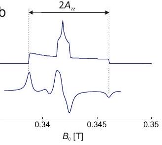
Figure 10.3: Construction of the solid-state EPR spectrum of a nitroxide at X band. (a) The absorption spectrum of each transition is considered separately. For , the hyperfine contribution vanishes and only anisotropy contributes. This line is the narrowest one at band. For the dispersion by anisotropy subtracts from the larger dispersion by hyperfine anisotropy. This line has intermediate width. For the dispersion from anisotropy adds to the dispersion from hyperfine anisotropy. This line has the largest width. (b) The three contributions from individual values add to the total EPR absorption spectrum (top). In CW EPR, the derivative of this absorption spectrum is observed (bottom). Because hyperfine anisotropy dominates, the separation between the outer extremities is .

In order to construct the solid-state spectrum, orientation dependence of the three transitions must be considered (Fig. 10.3(a)). At each individual orientation, the line is the center line. Since the hyperfine contributions scales with , it vanishes for this line and only anisotropy is observed. At X band, where hyperfine anisotropy dominates by far, this line is the narrowest one. The lineshape is the one for pure anisotropy (see Fig. 3.4). For , the orientation with the largest shift of the resonance field coincides with the one of smallest hyperfine shift. Hence, the smaller resonance field dispersion by anisotropy subtracts from the larger dispersion by hyperfine anisotropy. For , the situation is opposite and the two dispersions add. Hence, the transition, which at any given orientation is the high-field line, has the largest resonance dispersion, whereas the low-field transition has intermediate resonance field dispersion. The central feature in the total absorption spectrum (Fig. ) is strongly dominated by the transition, whereas the outer shoulders correspond to the (low field) and (high field) transitions at the orientation. Therefore, the splitting between the outer extremities in the CW EPR spectrum, which correspond to these shoulders in the absorption spectrum, is .

18.1.4. Influence of dynamics on the nitroxide spectrum

In liquid solution, molecules tumble stochastically due to Brownian rotational diffusion. In the following we consider isotropic rotational diffusion, where the molecule tumbles with the same average rate about any axis in its molecular frame. This is a good approximation for nitroxide spin probes with small substituents . For instance, TEMPO with is almost spherical with a van-der-Waals radius of ÅÅ. In water at ambient temperature, the rotational correlation time for TEMPO is of the order of . The product with the maximum anisotropy of the nitroxide EPR spectrum on an angular frequency axis is much smaller than unity. In this situation, anisotropy averages and three narrow lines of equal width and intensity are expected. The spectrum in Fig. 10.2(a) corresponds to this situation and a closer look reveals that the high-field line has somewhat lower amplitude. This can be traced back to a larger linewidth than for the other two lines, which indicates a shorter for the transition than for the other transitions. Indeed, transverse relaxation is dominated by the effect from combined hyperfine and anisotropy, which is largest for the transition that has the largest anisotropic dispersion of resonance frequencies. With increasing rotational correlation time , one expects this relaxation process to become stronger, which should lead to more line broadening that is strongest for the high-field line and weakest for the central line. This is indeed observed in the simulation for ns shown in the bottom trace of Fig. .

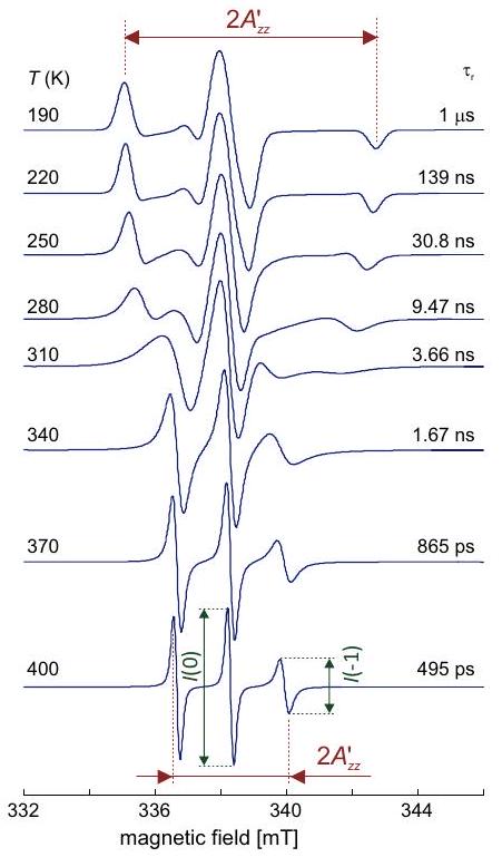
Figure 10.4: Simulation of X-band CW EPR spectra of an isotropically tumbling nitroxide radical for different rotational correlation times . A rotational correlation time of s at and an activated process with activation energy of were assumed, close to parameters observed for TEMPO in a synthetic polymer.

According to Kivelson relaxation theory, the ratio of the line width of one of the outer lines to the line width of the central line is given by

where

and

with the hyperfine anisotropy parameter

and the electron Zeeman anisotropy parameter

The relaxation time for the central line can be computed from the corresponding peak-topeak linewidth in field domain as

Thus, Eqs. (10.1-10.3) can be solved for the only remaining unknown . In practice, ratios of peak-to-peak line amplitudes are analyzed rather than linewidth ratios, as they can be measured with higher precision. The linewidth ratio is related to the amplitude ratio (see bottom trace in Fig. 10.4) in a first derivative spectrum by

since the integral intensity of the absorption line (double integral of the derivative lineshape) is the same for each of the three transitions. The rotational correlation time can thus be determined by, e.g.,

where is the peak-to-peak linewidth of the central line. This equation can be applied in the fast tumbling regime, where the three individual lines for , and can still be clearly recognized and have the shape of symmetric derivative absorption lines.

For slower tumbling with , the line shape becomes more complex and approaches the rigid limit (solid-state spectrum) at about (Fig. 10.4). These lineshapes can be simulated by considering multi-site exchange between different orientations of the molecule with respect to the magnetic field. Unlike for two-site exchange, which is discussed in the NMR part of the lecture course (see Section 3 of the NMR lecture notes), no closed expressions can be obtained for multi-site exchange. Nevertheless we can estimate the time scale where the spectral features are broadest and transverse relaxation times are shortest. Coalescence for two-site exchange is observed at . By substituting by by the maximum anisotropy of , corresponding to , we find a "coalescence time" ns. The simulations in Fig. show indeed that around this rotational correlation time, the

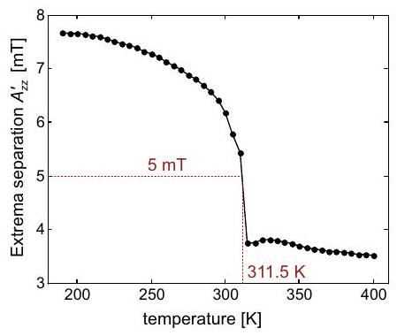
Figure 10.5: Plot of the outer extrema separation as a function of temperature for nitroxide spectra simulated under the same assumptions as in Fig. 10.4.

character of the spectrum changes from fast orientation exchange (liquid-like spectrum with three distinct peaks) to slow orientation exchange (solid-like spectrum).

A simple way of analyzing a temperature dependence, such as the one shown in Fig. 10.4, is to plot the outer extrema separation as a function of temperature (Fig. 10.5). The "coalescence time" in such a plot corresponds to the largest gradient , which coincides with the mean between the values in the fast tumbling limit and rigid limit, which is . In the case at hand, this coalescence time is and is observed at a temperature . The temperature is the temperature where the material becomes "soft" and molecular conformations can rearrange. Nitroxide spectra in the slow tumbling regime can reveal more details on dynamics, for instance, whether there are preferred rotation axes, whether motion is restricted due to covalent linkage of the nitroxide to a large molecule, or whether there is local order, such as in a lipid bilayer.

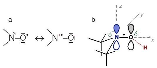
Figure 10.6: Influence of polarity of the environment and of hydrogen bonding on shift and hyperfine coupling. (a) In the mesomeric structure where the unpaired electron is on the oxygen atom (left), five valence electrons are formally assigned to and six to , which corresponds to electroneutrality. In the mesomeric structure where the unpaired electron is on the nitrogen atom (right), only four valence electrons are formally assigned to and seven to , which corresponds to a positive charge at and to a negative charge at . (b) Admixture of the charge-separated mesomeric structure generates partial charges and is favored in a polar environment that screens Coulomb attraction of the two charges. Hydrogen bonding to oxygen lowers energy of the lone pair, making excitation of a lone pair electron to the SOMO less likely, and thus decreasing shift.

18.1.5. Polarity and proticity

Delocalization of the unpaired electron in the group can be understood by considering mesomeric structures (Fig. 10.6). If the unpaired electron resides on oxygen, the formal number of valence electrons is five on nitrogen and six on oxygen, corresponding to the nuclear charge that is not compensated by inner shell electrons. Hence, both atoms are formally neutral in this limiting structure. If, on the other hand, the unpaired electron resides on the nitrogen atom, only four valence electrons are assigned to this atom, whereas seven valence electrons are assigned to the oxygen atom. This corresponds to charge separation with the formal positive charge on nitrogen and the formal negative charge on oxygen. The charge-separated form is favored in polar solvents, which screen Coulomb attraction between the two charges, whereas the neutral form is favored in nonpolar solvents. Hence, for a given nitroxide radical in a series of solvents, the hyperfine coupling, which stems from spin density on the nitrogen atom, is expected to increase with increasing solvent polarity. This effect has indeed been found. It is most easily seen in the solid state for but can also be discerned in the liquid state for .

The change in is expected to be anti-correlated to the shift, because this shift arises from SOC at the oxygen atom and, the higher spin density on the nitrogen atom is, the lower it is on the oxygen atom. This effect has also been found and is most easily detected by high-field/high-frequency EPR at frequencies of W-band frequencies of or even higher frequencies. How is correlated to depends on proticity of the solvent. Protic solvents form hydrogen bonds with the lone pairs on the oxygen atom of the N-O group. This lowers energy of the lone pair orbitals, making excitation of an electron from these orbitals to the SOMO less likely. Since this excitation provides the main contribution to SOC and thus to shift, hydrogen bonding to oxygen reduces shift. If two nitroxides have the same hyperfine coupling in an aprotic and protic environment, will be lower in the protic environment. This effect has also been found. In some cases it was possible to discern nitroxide labels with zero, one, and two hydrogen bonds by resolution of their features in W-band CW EPR spectra. Slopes of for aprotic at for protic environments have been found for the correlation between and for MTSL in spin-labeled bacteriorhodopsin in lipid bilayers [Ste+00].

19. Water accessibility

Polarity and proticity are proxy parameters for water accessibility of spin-labeled sites in proteins. Two other techniques provide complementary information. First, water can be replaced by deuterated water and the modulation depth of deuterium ESEEM can be measured. Because of the dependence of modulation depth (see Eq. (8.7)) the technique is most sensitive to deuterium nuclei in the close vicinity of the spin label. As long as , modulation depth contributions of individual nuclei add, so that the total deuterium modulation depth is a measure for local deuterium concentration close to the label. Data can be processed in a way that removes the contribution from directly hydrogen-bonded nuclei. Strictly speaking, this technique measures the concentration of not only water protons but also the one of any exchangeable protons near the label, but only to the extent that these exchangeable protons are water accessible during sample preparation or measurement.

A second, more direct technique that is applicable at ambient temperature measures the proton NMR signal as a function of irradiated microwave power with the microwave frequency being on-resonant with the central transition of a nitroxide spin label. Such irradiation transfers electron spin polarization to water protons by the Overhauser effect. This Overhauser dynamic nuclear polarization (DNP) is highly specific to water, as it critically depends on the water proton NMR signal being narrow and on fast diffusion of water. In biomolecules, water accessibility of spin labels is high at water-exposed surfaces of soluble and membrane proteins and low inside the proteins and at lipid-exposed surfaces. For transporters, water accessibility can change with state in the transport process.

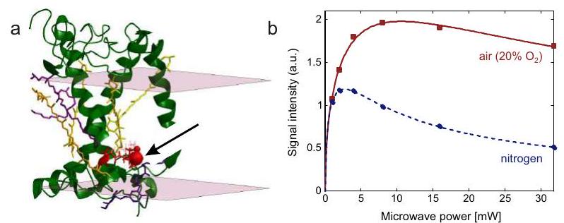
Figure 10.7: Characterization of oxygen accessibility at spin-labeled site V229C in major plant light harvesting complex LHCII by CW progressive power saturation. (a) Ribbon model of LHCII with green with its carotenoid cofactors (yellow, violet) and space-filling model of residue 229 (red, marked by an arrow). The pink planes correspond to the lipid headgroup layer of the thylakoid membrane in chloroplasts. (b) Progressive power saturation curves in the absence (blue) and presence (red) of oxygen.

19.1.6. Oxygen accessibility

Since collision of paramagnetic triplet oxygen with spin probes enhances relaxation (Fig. , the saturation parameter is smaller for oxygen-accessible spin labels than for spin labels not accessible to oxygen. This change can be detected by CW progressive power saturation measurements (Section 7.2.2). The experiment is most conveniently performed with capillary tubes made of the gas permeable plastic TPX. A reference measurement is performed in a nitrogen atmosphere, which causes deoxygenation of the sample on the time scale of 15 min. The gas stream is then changed to air (20% oxygen) or pure oxygen and the measurement is repeated. Such data are shown in Fig. for residue 229 in major plant light harvesting complex LHCII. This residue is lipid exposed. As a nonpolar molecule, oxygen dissolves well in the alkyl chain region of a lipid bilayer. Accordingly, the signal saturates at higher power in an air atmosphere than in a nitrogen atmosphere. Oxygen accessibility can be quantified by a normalized parameter (Section 7.2.2).

20. Local pH measurements

The hyperfine coupling of nitroxide spin probes becomes sensitive if the heterocycle that contains the group also contains a nitrogen atom that can be protonated in the desired range. This applies, for instance, to the imidazolidine nitroxide 3 in Fig. , which has a pK value of and exhibits a change in isotropic N hyperfine coupling of between the protonated (1.43 mT) and deprotonated form, which can be resolved easily in liquid solution. By modifying the probe to a label, local can be measured near a residue of interest in a protein.

21. Spin traps

Many radicals are very reactive. This fact makes their detection during chemical reactions and in living cells very important, but it also makes their concentration very low, since often their formation reaction is slower than the reactions that destroy them again. For instance, concentration of the hydroxyl radical , a reactive oxygen species (ROS) in living cells, is too low for EPR detection even under conditions where leads to cell damage or cell death. The situation is somewhat better for the superoxide anion radical , but physiologically relevant concentrations are hard to detect also for this species.

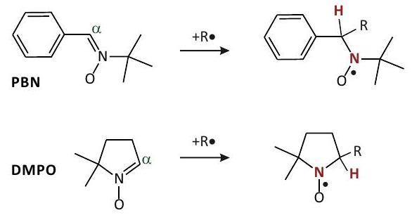
Figure 10.8: Reaction of the commonly used spin traps phenylbutylnitrone (PBN) and 5,5-dimethyl-1pyrroline N-oxide (DMPO) with unstable radicals . Hyperfine couplings of the and atom of the formed nitroxide (red) as well as the value of the nitroxide provide fingerprint information on the type of radical .

ROS and some other highly reactive radicals of interest are most easily detected by spin trapping. A spin trap (Fig. 10.8) is a diamagnetic compound that is primed to form a stable radical by reaction with an unstable radical. The most frequently used spin traps are nitrones that form nitroxide radicals by addition of the unstable radical to the atom in position of the nitrone group. The formed nitroxide radicals are not as stable as the ones used as spin labels, mainly because they contain a hydrogen atom in position to the group. Their lifetime is usually on the minute time scale, which is sufficient for detection. The hyperfine coupling of the atom is sensitive to the type of primary radical , i.e. to the nature of the other substituent at the atom. Furthermore, these nitrones are less sterically crowded than the ones that would yield more stable nitroxides and thus the nitrones are more reactive and trap radicals more easily. In addition to the hyperfine coupling, the hyperfine coupling of the atom of the group is sensitive to the nature of . A database of experimental results supports assignment of in difficult cases: http://tools . niehs . nih.gov/stdb/index. .

Look a the "Hints for Using the Spin Trap Database" before you start your search. The keyword format is powerful, but not very intuitive.

22. Bibliography

23. Books

[CCM16] V. Chechik, E. Carter, and D. M. Murphy. Electron Paramagnetic Resonance. Ed. Oxford: Oxford University Press, 2016 (cited on pages 8, 26).

[KBE04] M. Kaupp, M. Buhl, and V. G. Malkin (Eds.) Calculation of NMR and EPR Parameters: Theory and Applications. Ed. Weinheim: Wiley-VCH, cited on page 16).

[Rie07] Philip Rieger. Electron Spin Resonance. Analysis and Interpretation. The Royal Society of Chemistry, 2007, P001-173. ISBN: 978-0-85404-355-2. DOI: 10.1039/ 9781847557872 . URL: http://dx. doi .org/10.1039/9781847557872 (cited on page 37).

[WBW94] J. A. Weil, J. R. Bolton, and J. E. Wertz. Electron Paramagnetic Resonance. Ed. New York: John Wiley & Sons, Inc., 1994 (cited on page 8).

24. Articles

[Cas+60] Theodore Castner et al. "Note on the Paramagnetic Resonance of Iron in Glass". In: J. Chem. Phys. , pages 668-673. Dor: http://dx. doi . org/10. (cited on page 40 .

[KM85] A. K. Koh and D. J. Miller. "Hyperfine coupling constants and atomic parameters for electron paramagnetic resonance data". In: Atomic Data and Nuclear Data Tables 33 (1985), pages 235-253 (cited on pages 22,23 ).

[Lef67] R. Lefebvre. "Pseudo-hyperfine interactions in radicals". In: Molecular Physics (1967), pages 417-426. Dor: (cited on page 22).

[Ste+00] Heinz-Jürgen Steinhoff et al. "High-field EPR studies of the structure and conformational changes of site-directed spin labeled bacteriorhodopsin". In: Biochim. Biophys. - Bioenergetics 1457 (2000), pages 253-262. DOI: 10. 1016/S0005 (cited on page 82 ).

25. Index

Davies ENDOR ..................... 59

dead time

DEER .............................. 68

form factor

DNP ............................. 82

dynamic nuclear polarization............82

Fermi contact interaction

g value

free electron

H

high-field approximation

high-field approximation

homogeneous linewidth

Hund's rule......................37

hyperfine contrast selectivity

Kramers ions ..................... 37

Kramers theorem

curve

level energies

first order

linear regime

M

modulation depth

ESEEM ....................62 molecular orbital

orientation selection

PELDOR ........................68

progressive power saturation ............55

quantum number

magnetic

spin

26.

rapid scan

reactive oxygen species

regularization parameter ............ 72

27. S

saturation curve

selection rule

site-directed spin labeling ............75

SOMO .......................11

spin packet

spin-orbit coupling

28. T

Tikhonov regularization

two-pulse ESEEM

29.

zero-field splitting.

Exporting to DOCX

epr_pciv_compressed.docx