2.6: Electron Tunneling

As we have seen several times already, solutions to the Schrödinger equation display several properties that are very different from what one experiences in Newtonian dynamics. One of the most unusual and important is that the particles one describes using quantum mechanics can move into regions of space where they would not be allowed to go if they obeyed classical equations. We call these classically forbidden regions. Let us consider an example to illustrate this so-called tunneling phenomenon. Specifically, we think of an electron (a particle that we likely would use quantum mechanics to describe) moving in a direction we will call \(R\) under the influence of a potential that is:

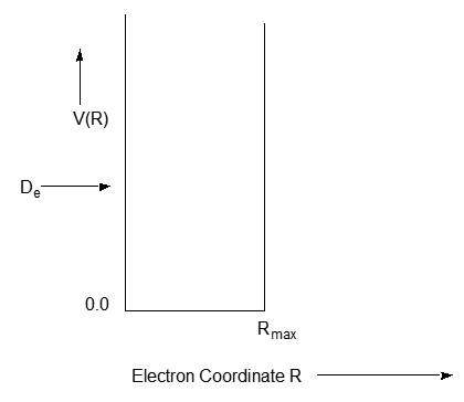
1. Infinite for \(R < 0\) (this could, for example, represent a region of space within a solid material where the electron experiences very repulsive interactions with other electrons);
2. Constant and negative for some range of \(R\) between \(R = 0\) and \(R_{\rm max}\) (this could represent the attractive interaction of the electrons with those atoms or molecules in a finite region or surface of a solid);
3. Constant and repulsive (i.e., positive) by an amount \(\delta V + D_e\) for another finite region from \(R_{\rm max}\)​ to \(R_{\rm max} +\delta\) (this could represent the repulsive interactions between the electrons and a layer of molecules of thickness d lying on the surface of the solid at \(R_{\rm max}\)​);
4. Constant and equal to \(D_e\) from \(R_{\rm max} +\delta\) to infinity (this could represent the electron being removed from the solid, but with a work function energy cost of \(D_e\), and moving freely in the vacuum above the surface and the ad-layer). Such a potential is shown in Figure 2.18.

Figure 2.18. One-dimensional potential showing a well, a barrier, and the asymptotic region.

The piecewise nature of this potential allows the one-dimensional Schrödinger equation to be solved analytically. For energies lying in the range \(D_e < E < D_e +\delta V\), an especially interesting class of solutions exists. These so-called resonance states occur at energies that are determined by the condition that the amplitude of the wave function within the barrier (i.e., for \(0 \le R \le R_{\rm max}\) ) be large. Let us now turn our attention to this specific energy regime, which also serves to introduce the tunneling phenomenon.

\[k=\sqrt{\dfrac{2m_e E}{\hbar^2}},k'=\sqrt{\dfrac{2m_e (E-D_e)}{\hbar^2}},\kappa'=\sqrt{\dfrac{2m_e (D_e+\delta V-E)}{\hbar^2}}\]

The piecewise solutions to the Schrödinger equation appropriate to the resonance case are easily written down in terms of sin and cos or exponential functions, using the following three definitions:

The combination of \(\sin(kR)\) and \(\cos(kR)\) that solve the Schrödinger equation in the inner region and that vanish at \(R=0\) (because the function must vanish within the region where \(V\) is infinite and because it must be continuous, it must vanish at \(R=0\)) is:

\[\psi = A\sin(kR) \hspace{1cm} (\text{for }0 \le R \le R_{\rm max} ).\]

Between \(R_{\rm max}\) and \(R_{\rm max} +\delta\), there are two solutions that obey the Schrödiger equation, so the most general solution is a combination of these two:

\[\psi = B^+ \exp(\kappa'R) + B^- \exp(-\kappa'R) \hspace{1cm} (\text{for }R_{\rm max} \le R \le R_{\rm max} +\delta).\]

Finally, in the region beyond \(R_{\rm max} +\delta\), we can use a combination of either \(\sin(k’R)\) and \(\cos(k’R)\) or \(\exp(ik’R)\) and \(\exp(-ik’R)\) to express the solution. Unlike the region near \(R=0\), where it was most convenient to use the sin and cos functions because one of them could be “thrown away” since it could not meet the boundary condition of vanishing at \(R=0\), in this large-\(R\) region, either set is acceptable. We choose to use the \(\exp(ik’R)\) and

\(exp(-ik’R)\) set because each of these functions is an eigenfunction of the momentum operator\(-ih\dfrac{∂}{∂R}\). This allows us to discuss amplitudes for electrons moving with positive momentum and with negative momentum. So, in this region, the most general solution is

\[\psi = C \exp(ik'R) + D \exp(-ik'R) \hspace{1cm} (\text{for }R_{\rm max} +\delta \le R < \infty).\]

There are four amplitudes (\(A, B^+, B^-,\) and \(C\)) that can be expressed in terms of the specified amplitude \(D\) of the incoming flux (e.g., pretend that we know the flux of electrons that our experimental apparatus shoots at the surface). Four equations that can be used to achieve this goal result when \(\psi\) and \(\dfrac{d\psi}{dR}\) are matched at \(R_{\rm max}\) and at \(R_{\rm max} + \delta\) (one of the essential properties of solutions to the Schrödinger equation is that they and their first derivative are continuous; these properties relate to y being a probability and the momentum \(-ih\dfrac{∂}{∂R}\) being continuous). These four equations are:

\[A\sin(kR_{\rm max}) = B^+ \exp(\kappa'R_{\rm max}) + B^- \exp(-\kappa'R_{\rm max}),\]

\[Ak\cos(kR_{\rm max}) = \kappa'​B^+ \exp(\kappa'​R_{\rm max}) - \kappa'​B^- \exp(-\kappa'R_{\rm max}),\]

\[B^+ \exp(\kappa'(R_{\rm max} + \delta)) + B^- \exp(-\kappa'(R_{\rm max} + \delta))\]

\[= C \exp(ik'(R_{\rm max} + \delta) + D \exp(-ik'(R_{\rm max} + \delta),\]

\[k'B^+ \exp(\kappa'(R_{\rm max} + \delta)) - k'B^- \exp(-\kappa'(R_{\rm max} + \delta))\]

\[= ik'C \exp(ik'(R_{\rm max} + \delta)) -ik' D \exp(-ik'(R_{\rm max} + \delta)).\]

It is especially instructive to consider the value of \(A/D\) that results from solving this set of four equations in four unknowns because the modulus of this ratio provides information about the relative amount of amplitude that exists inside the barrier in the attractive region of the potential compared to that existing in the asymptotic region as incoming flux.

The result of solving for \(A/D\) is:

\[\dfrac{A}{D} = \frac{4 \kappa'\exp(-ik'(R_{\rm max}+\delta))}{\exp(\kappa'\delta)(ik'-\kappa')(\kappa'\sin(kR_{\rm max})+k\cos(kR_{\rm max}))/ik'+ \exp(-\kappa'\delta)(ik'+\kappa')(\kappa'\sin(kR_{\rm max})-k\cos(kR_{\rm max}))/ik' }.\]

To simplify this result in a manner that focuses on conditions where tunneling plays a key role in creating the resonance states, it is instructive to consider this result under conditions of a high (large \(D_e + \delta V - E\)) and thick (large \(\delta\)) barrier. In such a case, the factor \(\exp(-\kappa'\delta)\) will be very small compared to its counterpart \(\exp(\kappa'\delta)\), and so

\[\dfrac{A}{D} = 4\frac{ik'\kappa'}{ik'-\kappa'} \frac{\exp(-ik'(R_{\rm max}+\delta)) \exp(-\kappa'\delta)}{\kappa'\sin(kR_{\rm max})+k\cos(kR_{\rm max}) }.\]

The \(\exp(-\kappa'\delta)\) factor in \(A/D\) causes the magnitude of the wave function inside the barrier to be small in most circumstances; we say that incident flux must tunnel through the barrier to reach the inner region and that \(\exp(-\kappa'\delta)\) governs the probability of this tunneling.

Keep in mind that, in the energy range we are considering (\(E < D_e+\delta\)), a classical particle could not even enter the region \(R_{\rm max} < R < R_{\rm max} + \delta\); this is why we call this the classically forbidden or tunneling region. A classical particle starting in the large-\(R\) region can not enter, let alone penetrate, this region, so such a particle could never end up in the \(0 <R < R_{\rm max}\) inner region. Likewise, a classical particle that begins in the inner region can never penetrate the tunneling region and escape into the large-\(R\) region. Were it not for the fact that electrons obey a Schrödinger equation rather than Newtonian dynamics, tunneling would not occur and, for example, scanning tunneling microscopy (STM), which has proven to be a wonderful and powerful tool for imaging molecules on and near surfaces, would not exist. Likewise, many of the devices that appear in our modern electronic tools and games, which depend on currents induced by tunneling through various junctions, would not be available. But, or course, tunneling does occur and it can have remarkable effects.

Let us examine an especially important (in chemistry) phenomenon that takes place because of tunneling and that occurs when the energy E assumes very special values. The magnitude of the \(A/D\) factor in the above solutions of the Schrödinger equation can become large if the energy E is such that the denominator in the above expression for \(A/D\) approaches zero. This happens when

\[\kappa'\sin(kR_{\rm max})+k\cos(kR_{\rm max})\]

or if

\[\tan(kR_{\rm max}) = - \frac{k}{\kappa}’.\]

It can be shown that the above condition is similar to the energy quantization condition

\[\tan(kR_{\rm max}) = - \frac{k}{\kappa}\]

that arises when bound states of a finite potential well similar to that shown above but with the barrier between \(R_{\rm max}\) and \(R_{\rm max} + \delta\) missing and with \(E\) below \(D_e\). There is, however, a difference. In the bound-state situation, two energy-related parameters occur

\[k =\sqrt{\dfrac{2\mu E}{\hbar^2}}\]

and

\[\kappa = \sqrt{\dfrac{2\mu (D_e-E)}{\hbar^2}} .\]

In the case we are now considering, \(k\) is the same, but

\[k' = \sqrt{\dfrac{2\mu (D_e+\delta V-E)}{\hbar^2}} \]

rather than \(\kappa\) occurs, so the two equations involving \(\tan(kR_{\rm max}) \)are not identical, but they are quite similar.

Another observation that is useful to make about the situations in which \(A/D\) becomes very large can be made by considering the case of a very high barrier (so that \(k'\) is much larger than \(k\)). In this case, the denominator that appears in \(A/D\)

\[\kappa'\sin(kR_{\rm max})+k\cos(kR_{\rm max}) \simeq \kappa' \sin(kR_{\rm max})\]

can become small at energies satisfying

\[\sin(kR_{\rm max}) \simeq 0.\]

This condition is nothing but the energy quantization condition that occurs for the particle-in-a-box potential shown in Figure 2.19.

Figure 2.19. One-dimensional potential similar to the tunneling potential but without the barrier and asymptotic region.

This potential is identical to the potential that we were examining for \(0 \le R \le R_{\rm max}\), but extends to infinity beyond \(R_{\rm max}\) ; the barrier and the dissociation asymptote displayed by our potential are absent.

Let’s consider what this tunneling problem\hbaras taught us. First, it showed us that quantum particles penetrate into classically forbidden regions. It showed that, at certain so-called resonance energies, tunneling is much more likely than at energies that are off-resonance. In our model problem, this means that electrons impinging on the surface with resonance kinetic energies will have a very high probability of tunneling to produce an electron that is highly localized (i.e., trapped) in the \(0 < R < R_{\rm max}\) region. Likewise, it means that an electron prepared (e.g., perhaps by photo-excitation from a lower-energy electronic state) within the \(0 < R < R_{\rm max}\) region will remain trapped in this region for a long time (i.e., will have a low probability of tunneling outward).

In the case just mentioned, it would make sense to solve the four equations for the amplitude C of the outgoing wave in the \(R > R_{\rm max}\) region in terms of the A amplitude. If we were to solve for \(C/A\) and then examine under what conditions the amplitude of this ratio would become small (so the electron cannot escape), we would find the same \(\tan(kR_{\rm max}) = - \dfrac{k}{\kappa}'\) resonance condition as we found from the other point of view. This means that the resonance energies tell us for what collision energies the electron will tunnel inward and produce a trapped electron and, at these same energies, an electron that is trapped will not escape quickly.

Whenever one has a barrier on a potential energy surface, at energies above the dissociation asymptote \(D_e\) but below the top of the barrier (\(D_e + \delta V\) here), one can expect resonance states to occur at special scattering energies \(E\). As we illustrated with the model problem, these so-called resonance energies can often be approximated by the bound-state energies of a potential that is identical to the potential of interest in the inner region (\(0 \le R \le R_{\rm max}\) ) but that extends to infinity beyond the top of the barrier (i.e., beyond the barrier, it does not fall back to values below \(E\)).

The chemical significance of resonances is great. Highly rotationally excited molecules may have more than enough total energy to dissociate (\(D_e\)), but this energy may be stored in the rotational motion, and the vibrational energy may be less than \(D_e\). In terms of the above model, high rotational angular momentum may produce a significant centrifugal barrier in the effective potential that characterizes the molecule’s vibration, but the system's vibrational energy may lie significantly below \(D_e\). In such a case, and when viewed in terms of motion on an angular-momentum-modified effective potential such as I show in Figure 2.20 , the lifetime of the molecule with respect to dissociation is determined by the rate of tunneling through the barrier.

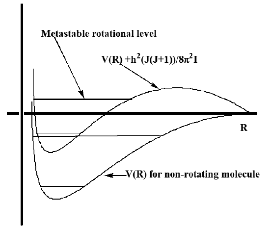
Figure 2.20. Radial potential for non-rotating (\(J = 0\)) molecule and for rotating molecule.

In this case, one speaks of rotational predissociation of the molecule. The lifetime t can be estimated by computing the frequency n at which flux that exists inside \(R_{\rm max}\) strikes the barrier at \(R_{\rm max}\)

\[\nu = \frac{\hbar k}{2\mu R_{\rm max}} \hspace{2cm} ({\rm sec})^{-1}\]

and then multiplying by the probability \(P\) that flux tunnels through the barrier from \(R_{\rm max}\) to \(R_{\rm max} + \delta\):

\[P = \exp(-2\kappa'\delta).\]

The result is that

\[\tau^{ -1}= \frac{\hbar k}{2\mu R_{\rm max}} \exp(-2\kappa'\delta)\]

with the energy \(E\) entering into \(k\) and \(\kappa'\) being determined by the resonance condition: (\kappa'\sin(kR_{\rm max})+k\cos(kR_{\rm max})) = minimum. We note that the probability of tunneling \(\exp(-2\kappa'\delta)\) falls of exponentially with a factor depending on the width d of the barrier through which the particle must tunnel multiplied by \(\kappa'\), which depends on the height of the barrier \(D_e + \delta\) above the energy \(E\) available. This exponential dependence on thickness and height of the barriers is something you should keep in mind because it appears in all tunneling rate expressions.

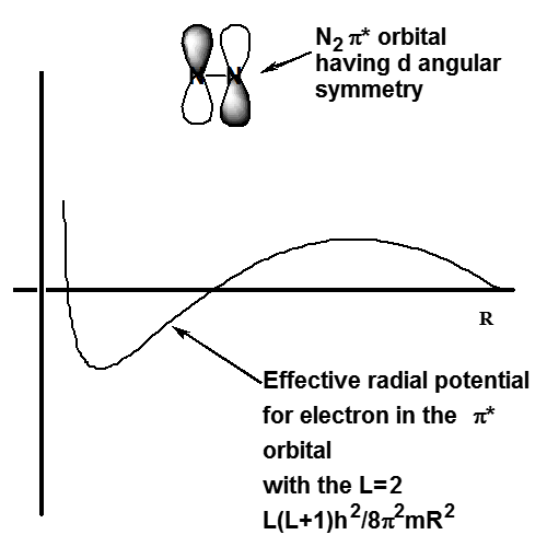
Another important case in which tunneling occurs is in electronically metastable states of anions. In so-called shape resonance states, the anion’s extra electron experiences an attractive potential due to its interaction with the underlying neutral molecule’s dipole, quadrupole, and induced electrostatic moments, as well as a centrifugal potential of the form \(\dfrac{L(L+1)\hbar^2}{8\pi^2m_eR^2}\) whose magnitude depends on the angular character of the orbital the extra electron occupies.

When combined, the above attractive and centrifugal potentials produce an effective radial potential of the form shown in Figure 2.21 for the \(N_2^-\) case in which the added electron occupies the \(\pi^*\) orbital which has \(L=2\) character when viewed from the center of the N-N bond. Again, tunneling through the barrier in this potential determines the lifetimes of such shape resonance states.

Figure 2.21 Effective radial potential for the excess electron in \(N_2^-\) occupying the \(\pi^*\) orbital which has a dominant \(L = 2\) component.

Although the examples treated above analytically involved piecewise constant potentials (so the Schrödinger equation and the boundary matching conditions could be solved exactly), many of the characteristics observed carry over to more chemically realistic situations. In fact, one can often model chemical reaction processes in terms of motion along a reaction coordinate (s) from a region characteristic of reactant materials where the potential surface is positively curved in all direction and all forces (i.e., gradients of the potential along all internal coordinates) vanish; to a transition state at which the potential surface's curvature along s is negative while all other curvatures are positive and all forces vanish; onward to product materials where again all curvatures are positive and all forces vanish. A prototypical trace of the energy variation along such a reaction coordinate is in Figure 2.22.

Figure 2.22. Energy profile along a reaction path showing the barrier through which tunneling may occur.

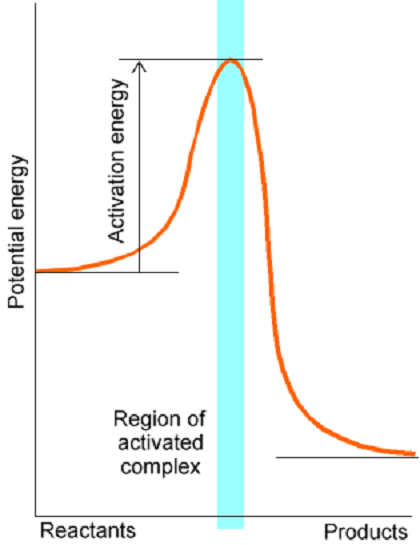
Near the transition state at the top of the barrier on this surface, tunneling through the barrier plays an important role if the masses of the particles moving in this region are sufficiently light. Specifically, if \(H\) or \(D\) atoms are involved in the bond breaking and forming in this region of the energy surface, tunneling must usually be considered in treating the dynamics.

Within the above reaction path point of view, motion transverse to the reaction coordinate is often modeled in terms of local harmonic motion although more sophisticated treatments of the dynamics is possible. This picture leads one to consider motion along a single degree of freedom, with respect to which much of the above treatment can be carried over, coupled to transverse motion along all other internal degrees of freedom taking place under an entirely positively curved potential (which therefore produces restoring forces to movement away from the streambed traced out by the reaction path). This point of view constitutes one of the most widely used and successful models of molecular reaction dynamics and is treated in more detail in Chapters 3 and 8 of this text.

Contributors and Attributions

Jack Simons (Henry Eyring Scientist and Professor of Chemistry, U. Utah) Telluride Schools on Theoretical Chemistry

Integrated by Tomoyuki Hayashi (UC Davis)