15.7: Chemical Potential, Activity, and Equilibrium

When we choose a standard state for the activity of a substance, we want the chemical potential that we calculate from the measured activity of a substance in a particular system to be the Gibbs free energy difference for the formation of the substance in that system from its constituent elements in their standard states.

Thus we must be able to measure the Gibbs free change for the process that produces the substance in its activity standard state from its constituent elements; this is the quantity that we designate as \({\Delta }_f{\tilde{G}}^o\left(A,ss\right)={\widetilde{\mu }}^o_A\). We must also be able to measure the difference between the chemical potential of the substance in this standard state and its chemical potential in the system of interest; this is the quantity that we designate as \(RT{ \ln {\tilde{a}}_A\ }\). The sum \[{\mu }_A={\widetilde{\mu }}^o_A+RT{ \ln {\tilde{a}}_A\ } \nonumber \]

is then the desired Gibbs free energy change for formation of the substance in the system of interest.

When it is convenient to choose the activity standard state to be the standard state of the pure liquid or the pure solid, we have

\[{\Delta }_f{\tilde{G}}^o\left(A,ss\right)={\widetilde{\mu }}^o_A={\Delta }_fG^o\left(A,\ell \right) \nonumber \] or \[{\Delta }_f{\tilde{G}}^o\left(A,ss\right)={\widetilde{\mu }}^o_A={\Delta }_fG^o\left(A,s\right) \nonumber \]

For other choices, we may be unable to measure the difference between the chemical potential of the substance in the activity standard state and that of its constituent elements in their standard states; that is, the value of \({\Delta }_f{\tilde{G}}^o\left(A,ss\right)={\widetilde{\mu }}^o_A\) may be unknown. Nevertheless, we can describe the Gibbs free energy changes in a cycle that goes from the elements in their standard states to the chemical species in the equilibrium system and back.

Figure 3. Relating activities in an equilibrium system to the Gibbs free energies of formation of the components in their activity standard states.

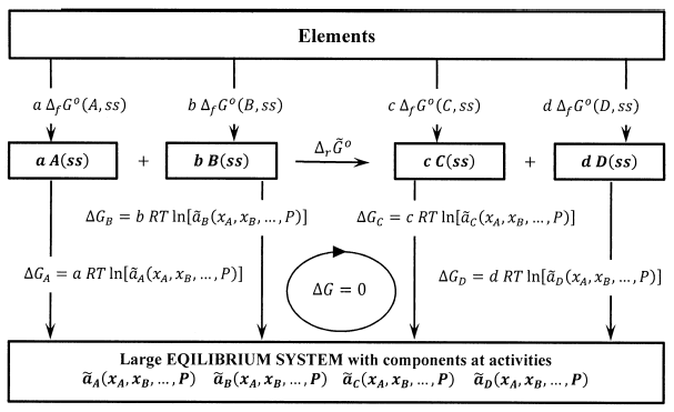
For the reaction \(aA+bB\to cC+dD\), this cycle is shown in Figure 3. Summing the Gibbs free energy changes in a clockwise direction around this cycle, we have

\[0=c\ {\Delta }_f{\tilde{G}}^o\left(C,ss\right)+d\ {\Delta }_f{\tilde{G}}^o\left(D,ss\right)-a\ {\Delta }_f{\tilde{G}}^o\left(A,ss\right)-b\ {\Delta }_f{\tilde{G}}^o\left(B,ss\right) \nonumber \] \[+c\ RT{ \ln {\tilde{a}}^c_C\ }+d\ RT{ \ln {\tilde{a}}^d_D\ }-a\ RT{ \ln {\tilde{a}}^a_A\ }-b\ RT{ \ln {\tilde{a}}^b_B\ } \nonumber \]

Writing \({\Delta }_r{\tilde{G}}^o\) to emphasize that the standard Gibbs free energy change for the reaction is now a difference between the chemical potentials of reactants and products in their activity standard states, we have

\[{\Delta }_r{\tilde{G}}^o=c\ {\Delta }_f{\tilde{G}}^o\left(C,ss\right)+d\ {\Delta }_f{\tilde{G}}^o\left(D,ss\right)-a\ {\Delta }_f{\tilde{G}}^o\left(A,ss\right)-b\ {\Delta }_f{\tilde{G}}^o\left(B,ss\right)={\Delta }_r{\widetilde{\mu }}^o \nonumber \]

and the equation for the Gibbs free energy change around the cycle becomes

\[{\Delta }_r{\tilde{G}}^o={\Delta }_r{\widetilde{\mu }}^o=-RT{ \ln \frac{{\tilde{a}}^c_C{\tilde{a}}^d_D}{{\tilde{a}}^a_A{\tilde{a}}^b_B}\ } \nonumber \]

Since the chemical reaction is at equilibrium, the activities term is constant. We have

\[K_a=\frac{{\tilde{a}}^c_C{\tilde{a}}^d_D}{{\tilde{a}}^a_A{\tilde{a}}^b_B} \nonumber \]

and \[K_a=\mathrm{exp}\left(\frac{-{\Delta }_r{\tilde{G}}^o}{RT}\right)=\mathrm{exp}\left(\frac{-{\Delta }_r{\widetilde{\mu }}^o}{RT}\right) \nonumber \]

We append the subscript, “\(a\)”, to indicate that the equilibrium constant, \(K_a\), is expressed in terms of the activities of the reacting substances. This cycle demonstrates the underlying logic for our calculation of \(K_a\) from our definition of activity, \({\mu }_A={\widetilde{\mu }}^o_A+RT{ \ln {\tilde{a}}_A\ }\), our definition of \({\Delta }_r\mu\), and the fact that

\[{\Delta }_r\mu =\sum^{\omega }_{j=1}{{\mu }_j{\nu }_j=0} \nonumber \]

is a criterion for equilibrium.

Introducing activity coefficients, we have

\[K_a=\frac{{\tilde{a}}^c_C{\tilde{a}}^d_D}{{\tilde{a}}^a_A{\tilde{a}}^b_B}=\left(\frac{c^c_Cc^d_D}{c^a_Ac^b_B}\right)\left(\frac{{\gamma }^c_C{\gamma }^d_D}{{\gamma }^a_A{\gamma }^b_B}\right) \nonumber \]

When we know \(K_a\) and can estimate the activity coefficients, we can predict the thermodynamic properties of a system whose component concentrations are known. In general, to determine \(K_a\) and the activity coefficients is more difficult than to determine the equilibrium concentrations. Over narrow ranges of concentrations it is often adequate to assume that the activity-coefficient function,

\[K_{\gamma }=\frac{{\gamma }^c_C{\gamma }^d_D}{{\gamma }^a_A{\gamma }^b_B} \nonumber \]

is approximately constant. When this is the case, the concentration function,

\[K_c=\frac{c^c_Cc^d_D}{c^a_Ac^b_B} \nonumber \]

is approximately constant. Then, a direct measurement of \(K_c\) in one equilibrium system makes it possible to predict the position of equilibrium in other similar systems.

The relationship between the equilibrium constant and the standard Gibbs free energy change for a reaction is extremely useful. If we can calculate the standard Gibbs free energy change from tabulated values, we can find the equilibrium constant and predict the position of equilibrium for a particular system. Conversely, if we can measure the equilibrium constant, we can find the standard Gibbs free energy change, \({\Delta }_r{\tilde{G}}^o\).

This brings us back to a central challenge in our development. We now have rigorous relationships between the Gibbs free energy and the fugacity or activity of a substance. To use these relationships, we must be able to relate the fugacity or activity to the concentration of a substance in any particular system that we want to study. For many common systems, this is difficult. In Chapter 16, we discuss some basic approaches to accomplishing it.