2.1: A Contrast of the Old and New Physics

Consider an electron of mass m = 9 ´ 10^-28 g which is confined to move on a line L cm in length. L is set equal to the approximate diameter of an atom, 1 ´ 10^-8cm = 1Å. Consider as well a system composed of a mass of 1 g confined to move on a line, say 1 metre in length. We shall apply quantum mechanics to the first of these systems and classical mechanics to the second.

Energy

As either mass moves from one end of its line to the other, the potential energy (the energy which depends on the position of the mass) remains constant. We may set the potential energy equal to zero, and all the energy is then kinetic energy (energy of motion). When the electron reaches the end of the line, we shall assume that it is reflected by some force. Thus at the ends of the line the potential energy rises abruptly to a very large value, so large that the electron can never "break through." We can plot potential energy versus position x along the line Fig. 2-1.

Fig. 2-1. Potential energy diagram for a particle moving on a line of lenght L. When the electron is at x = 0 or x = L the potential energy is infinite and for values of x between these limits (0< x < L ) the potential energy is zero.

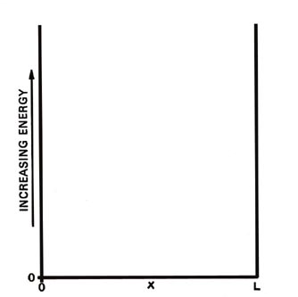
We refer to the electron (or the particle of m = 1 g) as being in a potential well and we can imagine the abruptly rising potential at x = 0 and x = L to be the result of placing a "wall" at each end of the line. First, what are the predictions of classical mechanics regarding the energy of the mass of 1 g? The total energy is kinetic energy and is simply:

\(E = KE = \frac{1}{2}mv^{2}\)

We know from experience that u, the velocity, can have any possible value from zero up to very large values. Since all values for u are allowed, all values for E are allowed. We conclude that the energy of a classical system may have any one of a continuous range of values and may be changed by any arbitrary amount. Let us contrast with this conclusion the prediction which quantum mechanics makes regarding the energy of an electron in a corresponding situation.

The quantum mechanical results are remarkable indeed, although they should not be surprising when we recall Bohr's explanation of the line spectra which are observed for atoms. Quantum mechanics predicts that there are only certain values of the energy which the electron confined to move on the line can possess. The energy of the electron is quantized. If this result could be observed for a massive particle, it would mean that only certain velocities were possible, say u = 1 cm/sec or 10 cm/sec but with no intermediate values! But then an electron is not really a particle. The expression for the allowed energies as given by quantum mechanics for this simple system is:

(1)

\[E_{n} = \frac{h^{2} n^{2}}{8mL^{2}} \nonumber \]

\(n = 1,2,3,4,....\)

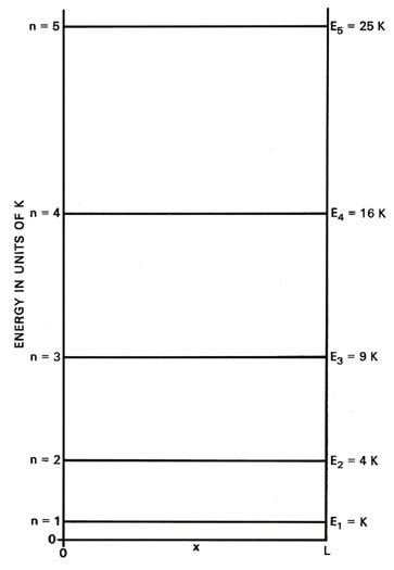
where again h is Planck's constant and n is an integer which may assume any value from one to infinity. Since only discrete values for E are possible, the appearance of the index n in equation (1) is necessary. A number such as n which appears in the expression for the energy is called a quantum number. Each value of the quantum number n fixes a value of E_n, one of the allowed energy values. We can indicate the possible values for the energy on an energy diagram. It is clear from equation (1) that for given values of m and L, E_n equals a constant (K = h²/8mL²) multiplied by n²:

(2)

\[E_{n} = Kn^{2} \nonumber \]

\(n = 1,2,3,4,....\)

Thus we can express the value of E_nin terms of so many units of K.

Each line, called an energy level, in Fig. 2-2 denotes an allowed energy for the system and the figure is called an energy level diagram. Each level is identified by its value of n as a subscript. A corresponding diagram for the case of the classical particle would consist of an infinite number of lines with infinitesimally small spacings between them, indicating that the energy in a classical system may vary in a continuous manner and may assume any value. The energy continuum of classical mechanics is replaced by a discrete set of energy levels in quantum mechanics.

Fig. 2-2. Energy level diagram for an electron moving on a line of length L. Only the first few levels are shown.

Suppose we could give the electron sufficient energy to place it in one of the higher (excited) energy levels. Then when it "fell" back down to the lowest value of E (called the ground level, E₁), a photon would be emitted. The energy e of the photon would be given by the difference in the values of E_n and E₁ and, since e = hv the frequency of the photon would be given by the relationship:

\[v = \frac{E_{n} - E_{1}}{h} \nonumber \]

\(n = 2,3,4,5,...\)

which is Bohr's frequency condition (I-4). Thus only certain frequencies would be emitted and the spectrum would consist of a series of lines.

We can illustrate the change in energy when the electron falls to the lowest energy level by connecting the upper level and the n = 1 level by an arrow in an energy level diagram. The frequency of the photon emitted during the indicated drop in energy is proportional to the length of the arrow, i.e., to the change in energy (Fig. 2-3). The line directly beneath each arrow represents the value of the frequency for that drop in energy. Since the differences in the lengths of the arrows increase as n increases, the separations between the observed frequencies show a corresponding increase. The spectrum, therefore, consists of a series of lines, with the spacings between the lines increasing as n increases. If the energy was not quantized and all values were possible, all jumps in energy would be possible and all frequencies would appear. Thus a continuum of possible energy values will produce a continuous spectrum of frequencies. A line spectrum, on the other hand, is a direct manifestation of the quantization of energy.

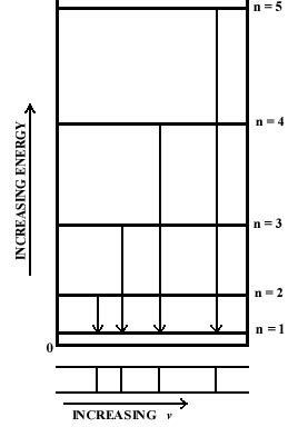Fig. 2-3. The origin of a line spectra.

In the quantum case, as in the classical case, all of the energy will be in the form of kinetic energy. We may obtain an expression for the momentum of the electron by equating the total value of the energy E_n to p²/2m, where p is the momentum
(= mu) of the electron, (p²/2m is another way of expressing 2mu².)

  \(E_{n} = \frac{n^{2}h^{2}}{8mL^{2}} = \frac{1}{2}mv^{2} = \frac{p^{2}}{2m}\)

This gives:

\(p = \pm \frac{nh}{2L}\)

\(n = 1,2,3,4,...\)

A plus and a minus sign must be placed in front of the number which gives the magnitude of the momentum to indicate that we do not know and cannot determine the direction of the motion. If the electron moves from left to right the sign will be positive. If it moves from right to left the sign will be negative. The most we can know about the momentum itself is its average value. This value will clearly be zero because of the equal probability for motion in either direction. The average value of p², however, is finite.

Since the lowest allowed value of the quantum number n in the quantum mechanical expression for the energy is unity, it is evident that the energy can never equal zero. A confined electron can never be motionless. The expression for E_n also indicates that the kinetic energy and the momentum increase as the length of the line L is decreased. Thus the kinetic energy and momentum of the electron increase as its motion becomes more confined. This is both an important and a general result and will be referred to again.

Position

The concept of a trajectory is fundamental to classical mechanics. Given a particular mass with a given initial velocity and a knowledge of the forces acting on it, we may use classical mechanics to predict the exact position and velocity of the particle at any future time. Thus we speak of the trajectory of the particle and we may calculate it to any desired degree of accuracy. It is also possible, within the framework of classical mechanics, to measure the position and velocity of a particle at any given instant of time. Thus classical mechanics correctly predicts what one can experimentally measure for massive particles.

We have previously mentioned the difficulties which are encountered when we attempt to determine the position of an electron. The results of the Compton effect indicate that part of the energy of the photon used in making the observation is transferred to the electron, and we invariably disturb the electron when we attempt to measure its position. Thus it is not surprising to find that quantum mechanics does not predict the position of an electron exactly. Rather, it provides only a probability as to where the electron will be found. When we consider the experiments which attempt to define the position of the electron, we shall find that this is the maximum information that can indeed be obtained even experimentally. The new mechanics again predicts only what can indeed be measured experimentally. We shall illustrate the probability aspect in terms of the system of an electron confined to motion along a line of length L. Quantum mechanical probabilities are expressed in terms of a distribution function which in this particular case we shall label P_n(x).

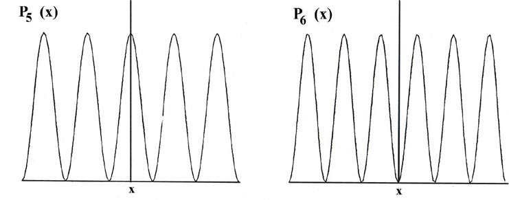
Consider the line of length L to be divided into a large number of very small segments, each of length Dx. Then the probability that the electron is in one particular small segment Dx of the line is given by the product of Dx and the value of the probability distribution function P_n(x) for that interval. For example, the probability distribution function for the electron when it is in the lowest energy level, n = 1, is given by P₁(x) (Fig. 2-4).

 

Fig. 2-4. Probability distributions P_n(x) for an electron confined to move on a line of fixed length in the quantum levels with n = 1, 2, ..., 6. The area of each rectangle shown in the figure for P₁(x) equals the probability that the electron is in the particular segment of the line Dx forming the base of the rectangle. The percentage shown in each rectangle is the percentage probability that the electron is in a particular segment Dx. The total probability that the electron is somewhere on the line is given by the total area under the P₁(x) curve, that is, by the sum of each small element of area P₁(x)Dx for each segment Dx. This total area is made to equal unity for every P_n(x) curve by expressing the values of P_n(x) in units of (1/L). Thus by definition a probability of one denotes a certainty.

The probability that the electron will be in the particular small interval Dx indicated in Fig. 2-4 is equal to the shaded area, an area which in turn is equal to the product of Dx and the average value of P₁(x) throughout the interval Dx, called P₁(x'),

  \(probability\ that\ electron\ is\ in\ segment \Delta x = P_{1}(x') \Delta x\)

The curve P₁(x) may be determined in the following manner. We design an experiment able to determine whether or not the electron is in one particular segment Dx of the line when it is known to be in the quantum level n = 1. (One way in which this might be done is described below.) We perform the experiment a large number of times, say one hundred, for each segment and record the ratio of the number of times the electron is found in a particular segment to the total number of observations made for that segment. For example, an electron is found to be in the segment marked Dx (of length 0.1 L) in the figure for P₁(x) in 18 out of 100 observations, or 18% of the time. In the other 82 observations the electron was in one of the other segments. Thus the average value of P₁(x) for this segment, called P₁(x') must be 1.8/L since P₁(x')Dx = (1.8/L) (0.1 L) = 0.18 or 18%. A similar set of experiments is made for each of the segments Dx and in each case a rectangle is constructed with Dx as base and with a height equal to P₁(x) such that the product P₁(x)Dx equals the fractional number of times the electron is found in the segment Dx. The limiting case in which the total length L is divided into a very large number of very small segments (Dx ® dx) would result in the smooth curve shown in the figure for P₁(x).

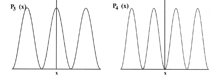
There is a different probability distribution for each value of E_n, or each quantum level, as shown, for example, by the probability distributions for the energy levels with n = 2, 3, 4, 5 and 6 (Fig. 2-4). The probability of finding the electron at the positions where the curve touches the x-axis is zero. Such a zero is termed a node. The number of nodes is always n-1 if we do not count the nodes at the ends of each P_n(x) curve.

Let us first contrast these results, particularly that for P₁(x), with the corresponding classical case. Since a classical analysis allows us to determine the position of a particle uniquely at any instant, either theoretically or experimentally, the idea of a probability distribution is foreign to a classical mechanical analysis. However, we still can determine the classical probability distribution for the particle confined to motion on a line. Since there are no forces acting on the particle as it traverses the line, it will be equally likely to be found at any point on the line (Fig 2-5). This probability will be the same regardless of the energy. There is again a striking difference between the classical and the quantum mechanics results. For the first quantum level, the graph of P₁(x) indicates the electron will most likely be found at the midpoint of the line. Furthermore, the form of P_n(x) changes with every change in energy. Every allowed value of the of the energy has associated with it a distinct probability distribution for the electron. Theses are the predictions of quantum mechanics regarding the position of a bound electron. Now let us investigate the experimental aspect of the problem to gain some physical reason for these predictions.

 

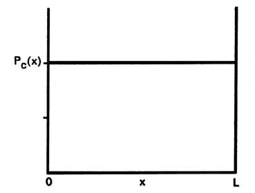Fig. 2-5. The classical probability distribution for motion on a line. This is the result obtained when the particle is located a large number of times at random time intervals. The classical probability function Pc(x) is the same for all values of x and equals 1/L, i.e., the particle is equally likely to be found at any value of x between 0 and L

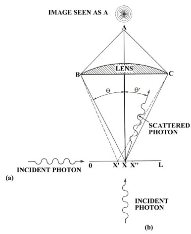
Let us design an experiment in which we attempt to pinpoint the position of an electron within a segment Dx. The experiment is a hypothetical one in that we imagine that we are to observe the electron through a microscope by reflecting or scattering light from it. Imagine the lens of a microscope being placed above the line L with the light entering from the side (Fig. 2-6 (a)). The electron, when illuminated with light, will act as a small source of light and will produce at A an image in the form of a bright disc surrounded by a group of rings of decreasing intensity. Because of this effect, which is entirely analogous to the diffraction effect observed for a pinhole source of light, the centre of the image will appear bright even if the electron is not precisely located at the point marked x. It could equally well have been at any value of x between the points x' and x" and produced an image visible to the eye at A if the difference in the path lengths Bx' and Cx' (or Bx" and Cx") is less than one half of a wavelength. In other words the resolving power of a microscope is not unlimited but is instead determined by the wavelength of the light used in making the observation. The use of the microscope imposes an inherent uncertainty in our observation of the position of the electron. With the condition that the difference in the path lengths to the outside rim of the lens must be no greater than one half a wavelength and with the use of some geometry, the magnitude of the uncertainty in the position of the electron, x'' - x' = Dx, is found to be given approximately by:

(3)	\[\Delta x \sim \frac{\lambda}{2 \sin \theta} \nonumber \]

where q is the angle indicated in the diagram.

 

Fig. 2-6. An idealized experiment for detecting the position of an electron.

Remembering the Compton effect and bearing in mind that we wish to disturb the electron as little as possible during the observation, we shall inquire as to the results obtained when a single photon is scattered from the electron. A single photon will not yield the complete diffraction pattern at A, but will instead produce a single flash of light. A diffraction pattern is the result of many photons passing through the microscope and represents the probability distribution for the emergent photons when they have been scattered by an electron lying between x' and x''. A single photon, when scattered from an electron within the length Dx, is however still diffracted and will produce a flash of light somewhere in one of the areas defined by the probability distribution produced by many photons passing through the system.

Thus even when we use but a single photon in our apparatus the uncertainty Dx in our experimentally determined position of the electron will still be given by equation (3). Obviously, if we want to locate an electron which is confined to move on a line to within a length that is small compared to the length of the line, we must use light which has a wavelength much less than L. This is exactly what equation (3) states: the shorter the wavelength of the light which is used to observe the electron, the smaller will be the uncertainty Dx. That being the case, why not do the experiment with light of very short wavelength compared to the length L, say l = (1/100)L? Then we can hope to find the electron on one small segment of the line, each segment being approximately (1/100)L in length. Let us calculate the frequency and energy of a photon which has the required wavelength of l = (1/100)L. As before, we set L equal to a typical atomic dimension of 1 x 10^-8 cm.

  \(\varepsilon = hv = \frac{hc}{\lambda} = \frac{6.6 \times 10^{-27} \times 3 \times 10^{10}}{10^{-10}} = 2.0 \times 10^{-6} ergs\)

We are immediately in difficulty, because the energy of the electron in the first quantum level is easily found to be:

  \(E_{1} = \frac{(6.6 \times 10^{-27})^{2}}{9.1 \times 10^{-28} \times 8 \times 10^{-16}} = 6.0 \times 10^{-11} ergs = K \)

The energy of the photon is approximately 1 x 10⁴ times greater than the energy of the electron! We know from the Compton effect that the collision of a photon with an electron imparts energy to the electron. Thus the electron after the collision will certainly not be in the state n = 1. It will be excited to oneCwe don't know whichCof the excited levels with n = 2 (E = 4K) or n = 3 (E = 9K), etc. The result is clear. If we demand an intimate knowledge of what the position of the electron is in a given state, we can obtain this information only at the expense of imparting to the electron an unknown amount of energy which destroys the system, i.e., the electron is no longer in the n = 1 level but in one of the other excited levels. If this experiment was repeated a large number of times and a record kept of the number of times an electron was located in each segment of the line (roughly (1/100)L), a probability plot similar to Fig. 2-4 would be obtained.

We can ask another kind of question regarding the position of the electron: "How much information can be obtained about the position of the electron in a given quantum level without at the same time destroying that level?" The electron cannot accept energy in an amount less than that necessary to excite it to the next quantum level, n = 2. The difference in energy between E₂, and E₁, is 3K. Thus if we are to leave the electron in a state of known energy and momentum we must use light whose photons possess an energy less than 3K.

Let us calculate the wavelength of the light with e = 2K and compare this value with the length L.

  \(\lambda = \frac{hc}{\varepsilon} = \frac{6.6 \times 10^{-27} \times 3.0 \times 10^{10}}{12 \times 10^{-11}} = 1.7 \times 10^{-6} cm\)

The wavelength is greater than the length of the line L. From equation (3) it is clear that the uncertainty in the position of the particle will be of the order of magnitude of, or greater than, L itself. The electron will appear to be blurred over the complete length of the line in a single experiment! Thus there are two interpretations which can be given to the probability distributions, depending on the experiment which is performed. The first is that of a true probability of finding the electron in a given small segment of the line using light of very short l relative to L. This experiment excites the electron, changes the system and leaves the electron with an unknown amount of energy and momentum. We have destroyed the object of our investigation. We now know where it was in a given experiment but not where it will be, in terms of energy or position.

Alternatively, we could use light with a l approximately equal to L. This does not excite the electron and leaves it in a known energy level. However, now the knowledge of the position is very uncertain. The photons are scattered from the system and give us directly the smeared distribution P₁ pictured in Fig. 2-4. In a real sense we must accept the fact that when the electron remains in a given state it is "smeared out" and "looks like" the pictures given for P_n. Thus we can interpret the P_n's as instantaneous pictures of the electron when it is bound in a known state, and forgot their probability aspect. This "smeared out" distribution is given a special name; it is called the electron density distribution. There will be a certain fraction of the total electronic charge at each point on the line, and when we consider a system in three dimensions, there will be a certain fraction of the total electronic charge in every small volume of space. Hence it is given the name electron density, the amount of charge per unit volume of space. The P_n's represent a charge density distribution which is considered static as long as the electron remains in the nth quantum level. Thus the P_n functions tell us either (a) the fraction of time the electron is at each point on the line for observations employing light of short wavelength, or (b) they tell us the fraction of the total charge found at each point on the line (the whole of the charge being spread out) when the observations are made with light of relatively long wavelength.

The electron density distributions of atoms, molecules or ions in a crystal can be determined experimentally by X-ray scattering experiments since X-rays can be generated with wavelengths of the same order of magnitude as atomic diameters (1 ´ 10^-8cm). In X-ray scattering the intensity of the scattered beam and the angle through which it is scattered are measured. The distribution of negative charge within the crystal scatters the X-rays and determines the intensity and angle of scattering. Thus these experimental quantities can be used to calculate the form of the electron density distribution.

There is a definite quantum mechanical relationship governing the magnitudes of the uncertainties encountered in measurements on the atomic level. We can illustrate this relationship for the one-dimensional system. Let us consider the minimum uncertainty in our observations of the position and the momentum of the electron moving on a line obtained in an experiment which leaves the particle bound in a given quantum level, say n = 1. This will require the use of light with l ~ L. We have seen that the use of light of this wavelength limits us to stating that the electron is somewhere on the line of length L. We can say no more than this with certainty unless we use light of much shorter l , and then we will change the quantum number of the electron. The uncertainty in the value of the position coordinate, which we shall call Dx, is just L, the length of the line:

  \(\Delta x = L\)

We have previously shown that the momentum of the electron in the nth quantum level is given by:

\(p_{n} = \pm \frac{nh}{2L}\)

\(n = 1,2,3, ...\)

the plus and minus signs denoting the fact that while we know the magnitude of the momentum we cannot determine whether the electron is moving from left to right (+nh/2L) or from right to left (-nh/2L). The minimum uncertainty in our knowledge of the momentum is the difference between these two possibilities, or for n = 1:

  \(\Delta p = + \frac{h}{2L} - (\frac{-h}{2L}) = \frac{H}{L}\)

The product of the uncertainties in the position and the momentum is:

  \(\Delta p \Delta x = L \frac{h}{L} = h\)

This result is a particular example of a general relationship governing the product of the uncertainties in the momentum and position known as Heisenberg's uncertainty principle. In the general case, the equality sign in the above equation is replaced by the symbol "³" which denotes that the product in the uncertainties DpDx equals or exceeds the value of Planck's contant h, that is, the general statement is given by DpDx ³ h.

If we endeavour to decrease the uncertainty in the position coordinate (i.e., make D x small) there will be a corresponding increase in the uncertainty of the momentum of the electron along the same coordinate, such that the product of the two uncertainties is always equal to Planck's constant. We saw this effect in our experiments wherein we employed light of short l to locate the position of the electron more precisely. When we did this we excited the electron to one of the other available quantum states, thus making a knowledge of the energy and hence the momentum uncertain. We might also try to defeat Heisenberg's uncertainty principle by decreasing the length of the line L. By shortening L, we would decrease the uncertainty as to where the electron is. However, as was noted previously, the momentum increases as L is decreased and the uncertainty in p is always the same order of magnitude as p itself; in this case twice the magnitude of p. Thus the decrease in Dx obtained by decreasing L is offset by the increase in Dp which accompanies the increased confinement of the electron; the product DxD p remains unchanged in value.

We can illustrate the operation of Heisenberg's uncertainty principle for a free particle by referring again to our hypothetical experiment in which we attempted to locate the position of an electron by using a microscope. We imagine the electron to be free and travelling with a known momentum in the direction of the x-axis with a photon entering from below along the y-axis. When the photon is scattered by the electron it may transfer momentum to the electron and continue on a line which makes an angle q' to the y-axis (Fig. 2-6). The photon, in doing so, will acquire momentum in the direction of the x-axis, a direction in which it initially had none. Since momentum must be conserved, the electron will receive a recoil momentum, a momentum equal in magnitude but opposite in direction to that gained by the photon. This is the Compton effect. Thus our act of observing the electron will lead to an uncertainty in its momentum as the amount of momentum transferred during the collision is uncontrollable. We may, however, set limits on the amount transferred and in this way determine the uncertainty introduced into the value of the momentum of the electron.

The momentum of the photon before the collision is all directed along the y-axis and has a magnitude equal to h/l . After colliding with the electron the photon may be scattered to the left or to the right of the y-axis through any angle q' lying between 0 and q and still be collected by the lens of the microscope and seen by the observer at A. Thus every photon which passes through the microscope will have an uncertainty of 2(h/l)sinq in its component of momentum along the x-axis since it may have been scattered by the maximum amount to the left and acquired a component of -(h/l)sinq or, on the other hand, it may have been scattered by the maximum amount to the right and acquired a momentum component of +(h/l)sinq. Any x-component of momentum acquired by the photon must have been lost by the electron and the uncertainty introduced into the momentum of the electron by the observation is also equal to 2(h/l)sinq .

In addition to the uncertainty induced in the momentum of the electron by the act of measurement, there is also an inherent uncertainty in its position (equation (3)) because of the limited resolving power of the microscope. The product of the two uncertainties at the instant of measurement or immediately following it is:

  \(\Delta p \Delta x \sim 2 \frac{h}{\lambda} \sin \theta \times \frac{\lambda}{2 \sin \theta} = h\)

Heisenberg's uncertainty relationship is again fulfilled. Our experiment employs only a single photon which, since light itself is quantized, represents the smallest packet of energy and momentum which we can use in making the observation. Even in this idealized experiment the act of observation creates an unavoidable disturbance in the system.

Degeneracy

We may use an extension of our simple system to illustrate another important quantum mechanical result regarding energy levels. Suppose we allow the electron to move on the x-y plane rather than just along the x-axis. The motions along the x and y directions will be independent of one another and the total energy of the system will be given by the sum of the energy quantum for the motion along the x-axis plus the energy quantum for motion along the y-axis. Two quantum numbers will now be necessary, one to indicate the amount of energy along each coordinate. We shall label these as n_x and n_y. Let us assume that the motion is confined to a length L along each axis, then:

\(E_{n_{x},{n_{y}}} = \frac{h^{2}}{8mL^{2}} n_{x}^{2} \ + \ \frac{h^{2}}{8mL^{2}} n_{y}^{2}\) \(= \frac{h^{2}}{8mL^{2}}(n_{x}^{2} + n_{y}^{2})\)

\(n_{x,y} = 1,2,3, ...\)

Nothing new is encountered when the electron is in the lowest quantum level for which n_x = n_y = 1. The energy E_1,1 simply equals 2h²/8mL².

Since two dimensions (x and y) are now required to specify the position of the electron, the probability distribution P_1,1(x,y) must be plotted in the third dimension. We may, however, still display P_1,1(x,y) in a two-dimensional diagram in the form of a contour map (Fig. 2-7). All points in the x-y plane having the same value for the probability distribution P_1,1(x,y) are joined by a line, a contour line. The values of the contours increase from the outermost to the innermost, and the electron, when in the leveln_x = n_y = 1, is therefore most likely to be found in the central region of the x-y plane.

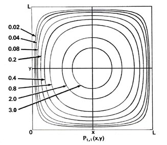
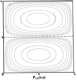
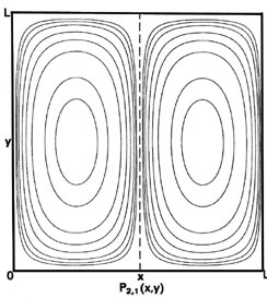
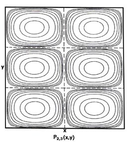
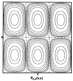
Fig. 2-7. Contour maps of the probability distributions P_{nx, ny} (x,y) for an electron moving on the x-y plane. The dashed lines represent the postion of nodes, lines along which the probability is zero. P_1,2 (x,y) and P_2,1 (x,y) are distributions for one doubly-degenerate level; P_2,3 (x,y) and P_3,2 (x,y) are examples of distributions for another degenerate level of still higher energy. The same contours are shown in each diagram and their values (in units of 4/L²) are indicated in the diagram for P_1,1(x,y).

A plot of P_1,1(x,y) along either of the axes indicated in Fig. 2-7 (one parallel to the x-axis at y = L/2 and the other parallel to the y-axis at x = L/2) is similar in appearance to that for P₁(x) shown in Fig. 2-4. That is, for a fixed value of y, the contribution to P_1,1(x,y) from the motion along the y-axis is constant and

  \(P_{1,1}(x,L/2) = constant \times P_{1}(x)\)

Thus, aside from the constant factor, P₁(x) provides a profile, or if P_1,1(x,y) were displayed in three dimensions, a cross section of the contour map of P_1,1(x). A contour map is a display of the probability or density distribution in a plane; a profile is a display of the density distribution along a line.

Now consider the possibility of n_x = 1 and n_y = 2. Then

  \(E_{1,2} = \frac{5h^{2}}{8mL^2}\)

We could also have the situation in which n_x = 2 and n_y = 1. This does not change the value of the total energy,

  \(E_{2,1} = E_{1,2} = \frac{5h^{2}}{8mL^{2}}\)

but the probability distributions (Fig. 2-7) are different, P_1,1(x,y) ¹P_2,1 (x,y). When n_x = 1 and n_y = 2, there must be a node on the y-axis, i.e., a zero probability of finding the electron at y = L/2. Thus a slice through P_1,2(x y) at x = L/2 parallel to the y-axis must be similar to the figure for P₂(x), while a slice parallel to the x-axis will still be similar to P₁(x). Just the reverse is true for the case n_x = 2 and n_y = 1. In this case, whether or not we can distinguish experimentally between the x- and y-axes, there are two different arrangements for the distribution of the electron, both of which have the same energy. The energy level is said to be degenerate. The degeneracy of an energy level is equal to the number of distinct probability distribution for the system, all of which belong to this same energy level.

The concept of degeneracy in an energy level has important consequences in our study of the electronic structure of atoms.