10.3: Computational Instructions

Start by creating a new file on your desktop and naming it cinnamic_acid. You should download the supporting files for this experiment and save them to the file that you just created. Start by opening cinnamic_coord.xyz in Avogadro and examining its structure, as shown in Figure 4.

Figure 4. Cinnamic acid geometry shown in Avogadro.

Next, you should open the input script, which you can find in the supporting files for this exercise, in notepad. This script contains the instructions for the computer to calculate the molecular orbitals of cinnamic acid. The text of the input file is very similar to that of previous exercises. It starts off with a # symbol, indicating a comment which describes calculation. The next line, which begins with a ! symbol, indicates the calculations and level of theory at which we want to perform the calculations. One difference from previous calculations is the inclusion of the LARGEPRINT keyword. This command directs the computer to include more information in the output file about the calculation than it usually would. Contained within this extra information are the molecular orbitals calculated during the computation. The last line begins with a * and indicates the coordinates file that the calculation will use.

Figure 5. Input script for the generation of molecular orbitals of cinnamic acid. Please note the name of the geometry input files, indicated by a red arrow, that you will need to change to ensure that it matches the name of your geometry file that you created.

We can now run our calculation using Orca via the command line as we did in previous exercises. Briefly, open the command prompt to your PC by right clicking on the start button and searching for command prompt. First, we need to tell the computer to look on the C drive and we do this by typing C: in the command prompt and hitting enter. Next, we need to tell the computer where the input script and the coordinates file are to run the calculation. We do this by typing cd (space) and pasting the file path into the command prompt. When you hit enter, the computer will paste a new line indicating that the current directory has changed, as shown in Figure 6A. To find the file path of your input script, right click on the input script (cinnamic.inp) and select properties. The file path will appear under location, and you can highlight and copy this file path (Figure 6 B).

Figure 6A. (Left) Changing of the file path in the command prompt to match the location of our input script. 6B. (Right) Locating the file path on the properties window of the input script (Red Arrow).

Next, we will run the calculation by typing orca cinnamic.inp > cinnamic.out and pressing enter in the command prompt. At first, it may not appear like anything is happening but the folder on your desktop housing the input file will quickly become populated with the output of your calculation. The calculations should take 30-45 minutes depending upon the speed of your computer and how many other processes your machine is running at the time.

After you have submitted your calculation, it is a good time for a cup of coffee or a nice walk! When the calculation is complete, your command prompt window will display a new line indicating it is ready for the next command.

Figure 7. Running the calculation using the command line. The line indicated by the red arrow shows the computer that we want to use Orca to calculate the commands in cinnamic.inp and that the results of this calculation should be placed in the output file cinnamic.out. The line indicated by the blue arrow is the computer indicating that the calculation is complete, and the command prompt is ready for the next command.

As shown in Figure 8, the folder where you put your initial coordinates file, is now populated with your experimental output.

Figure 8. The output of the molecular orbital calculation for cinnamic acid contained within the cinnamic acid file that you created.

To view the molecular orbitals of cinnamic acid you will first need to open the output file (has the .out file extension) with Avogadro to view the molecular orbitals of the species. As shown in Figure 9, the output file will show the molecular orbitals in the upper right portion of the screen.

Figure 9. The output file of cinnamic acid loaded in Avogadro. The surface button is indicated by a red arrow.

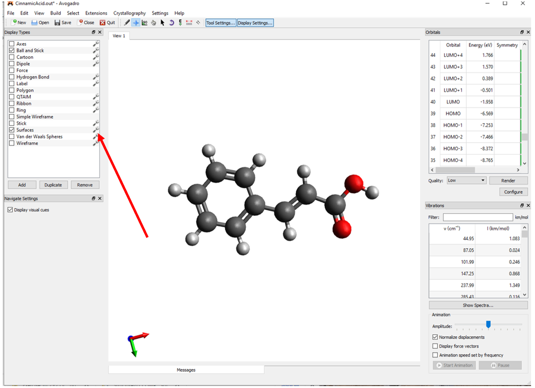
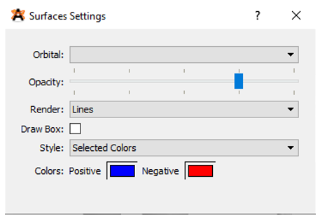
Before you view any of the molecular orbitals you will need to click on the wrench button adjacent to the surfaces. From the surface settings window that appears you can change the positive and negative surfaces to blue and red respectively (Figure 10). Also, to make the orbitals easier to see you should change the background color by clicking View🡪Set Background Color🡪White.

Figure 10. Setting the surface colors (colors of the lobes of the molecular orbitals) to blue and red respectively.

You should now be able to click on the each of the molecular orbitals to examine them individually. Please note that the energy levels of each molecular orbital can be found in the panel in the top right of the Avogadro screen. You should now be able answer the questions at the end of the exercise.

References

1. Neese, F. Software Update: The ORCA Program System, Version 4.0. WIREs Comput. Mol. Sci. 2018, 8 (1), e1327. https://doi.org/10.1002/wcms.1327.
2. Neese, F. The ORCA Program System. WIREs Comput. Mol. Sci. 2012, 2 (1), 73–78. https://doi.org/10.1002/wcms.81.
3. Neese, F. Software Update: The ORCA Program System—Version 5.0. WIREs Comput. Mol. Sci. 2022, 12 (5). https://doi.org/10.1002/wcms.1606.
4. Neese, F.; Wennmohs, F.; Becker, U.; Riplinger, C. The ORCA Quantum Chemistry Program Package. J. Chem. Phys. 2020, 152 (22), 224108. https://doi.org/10.1063/5.0004608.
5. Hanwell, M. D.; Curtis, D. E.; Lonie, D. C.; Vandermeersch, T.; Zurek, E.; Hutchison, G. R. Avogadro: An Advanced Semantic Chemical Editor, Visualization, and Analysis Platform. J. Cheminformatics 2012, 4 (1), 17. https://doi.org/10.1186/1758-2946-4-17.
6. Avogadro: An Open-Source Molecular Builder and Visualization Tool. http://avogadro.cc/.
7. Liebermann, C. Ueber Cinnamylcocaïn. Berichte Dtsch. Chem. Ges. 1888, 21 (2), 3372–3376. https://doi.org/10.1002/cber.188802102223.
8. Nakamura, M.; Chi, Y.-M.; Yan, W.-M.; Nakasugi, Y.; Yoshizawa, T.; Irino, N.; Hashimoto, F.; Kinjo, J.; Nohara, T.; Sakurada, S. Strong Antinociceptive Effect of Incarvillateine, a Novel Monoterpene Alkaloid from Incarvillea s Inensis. J. Nat. Prod. 1999, 62 (9), 1293–1294. https://doi.org/10.1021/np990041c.