8.3: Computational Instructions

In this exercise we will be examining the energetics of the starting materials, transition state, and products of an E2 reaction in a solvent of water or DMSO. Specifically, we will be examining the energies associated with the E2 reaction between the methoxide anion and 2-chloro-2-methylpropane (Figure 2).

Figure 2. E2 elimination between the hydroxide anion and 2-chloro-2-methylpropane.

Up until this point, all of the calculations that we have performed have been in the gas phase. While this allows us to calculate energy levels and transitions states, these calculations don’t accurately reflect many organic reactions which occur in a solvent. Intermolecular attractions between a solvent and reactants, referred to as solvation, can have a dramatic effect on the energies of chemical species. When calculating the interaction of solvent with reactants, known as solvation, many programs will use what is referred to as implicit solvation. In this case, individual molecules of solvent are not modeled but rather the program considers the bulk properties of the solvent, such as the dielectric constant, when surrounding molecules of interest. The advantage to this type of modeling as opposed to the modeling of explicit solvent molecules is that it takes less computational power and time while providing reasonable results.

The dielectric constant of a solvent is a property which you may have been exposed to in a physics but isn’t always discussed explicitly in chemistry. Materials with a high dielectric constant are effective at shielding charges from each other. The force pushing apart two negative charges is much weaker if they are separated by a material with a high dielectric constant. Likewise, a positive and negative charge attract each other much more weakly in a high dielectric medium. Most polar solvents tend to have larger dielectric constants, and non-polar solvents tend to have smaller dielectric constants. By asking ORCA to use a specific solvent for a calculation, the program assumes that charged moieties have weaker or stronger effects depending on if it is a high or low dielectric solvent.

Computing the Energy of Reactants and Products

Despite using the computationally more efficient implicit solvation methods, calculating the energy values of starting materials, transition states, and products is time intensive for systems involving more than a few atoms. Because of this, you will be provided with energy values and geometry coordinate files for each step of the E2 reaction, shown below in Figure 3.

Figure 3A. Reaction scheme for the E2 reaction being modeled in this exercise.

Please note that the geometries that you will be provided with have been optimized in the indicated solvent while the energies you are provided are gas phase energies.Your goal in performing this exercise will be to compute the energy of solvation for each step of the reaction and use this information to create a reaction coordinate diagram comparing the E2 reaction in water and DMSO as a solvent.

Figure 3B. (Bottom) Summary of the gas phase energy values for the reaction. Please note that the values are slightly different for each condition because the geometries were determined in the indicated solvent.

	Starting Material	Transition State	Products
Energy in DMSO (Eh)	-693.3164355	-693.31569972	-693.38054907
Energy in \(H_2O\) (Eh)	-693.3416374	-693.32910367	-693.38044269

Start by creating a folder on the desktop of your computer and label it as solvation. Within this folder, please create the following subfolders: SM_DMSO, TS_DMSO, PR_DMSO, SM_H2O, TS_H2O, and PR_H2O. Next, you should download the supporting files for this exercise. These files will include a generic input script (denoted by a .inp file extension), and molecular coordinates for the geometry optimized starting materials, transition state and products (denoted by a .xyz file extension). Place a copy of the generic input file that you downloaded into each of the nested subfolders. Next you should place the molecular coordinates file for each step into its corresponding subfolder. A description of the file structure is shown in Figure 4.

Figure 4. Description of the nested files used in this exercise.

The process for computing the solvation energies of each of these steps is the same so we will walk you through the first calculation step-by-step and then allow you to perform the rest of the calculations using the same procedure. Specifically, we will work on calculating the solvation energy of the starting material in DMSO. Start by opening the starting coordinate files in Avogadro and check that the structure looks correct for the combination of the hydroxide anion and 2-chloro-2-methylpropane as shown in Figure 5.

Figure 5. Starting coordinates visualized in Avogadro.

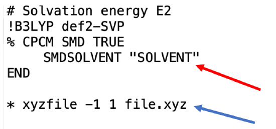
Next, you should rename the generic input file within the SM_DMSO subfolder. Save the generic input file as SM_DMSO.inp. You will then need to modify the generic input file so that it refers to the coordinate file within the starting_DMSO subfolder. Specifically, you should replace file.xyz in the input file with SMdmso.xyz. Additionally, you will need to change the SOLVENT keyword to the solvent that you want to model. In this case, you will change SOLVENT to DMSO, as shown in Figure 6. After you have made these changes, please be sure to save the file. When you compute structures later in water you can use the WATER keyword.

Figure 6. The generic input script for Orca. The SOLVENT keyword shown by a red arrow should be replaced with the solvent you are using. The generic coordinate file shown by a blue arrow, file.xyz, should be replaced with the coordinates that you are looking to calculate.

We can now run our calculation using Orca via the command line as we did in the previous exercise. Briefly, open the command prompt to your PC by right clicking on the start button and searching for command prompt. First, we need to tell the computer to look on the C drive and we do this by typing C: and hitting enter. Next, we need to tell the computer where the input script and the coordinates file are to run the calculation. We do this by typing cd (space) and pasting the file path. When you hit enter, the computer will paste a new line indicating that the current directory has changed, as shown in Figure 7A. To find the file path of your input script, right click on the input script (SM_DMSO.inp) and select properties. The file path will appear under location, and you can highlight and copy this file path (Figure 7B).

Figure 7A. (Left) Changing of the file path in the command prompt to match the location of our input script. 7B. (Right) Locating the file path on the properties window of the input script (Red Arrow).

Next, we will run the calculation by typing orca SM_DMSO.inp > SM_DMSO.out and pressing enter. At first it may not appear like anything is happening but the folder on your desktop labeled SM_DMSO will quickly become populated with the output of your calculation. Depending upon the speed of your computer the calculation will take from 1-5 minutes, and upon completion the command prompt will print another line indicating that it is ready for the next command (Figure 8).

Figure 8. Running the calculation using the command line. The line indicated by the red arrow shows the computer that we want to use Orca to calculate the commands in SM_DMSO.inp and that the results of this calculation should be placed in the output file SM_DMSO.out. The line indicated by the blue arrow is the computer indicating that the calculation is complete, and the command prompt is ready for the next command.

Correcting Energies for Solvation

As mentioned above, a correction needs to be applied to the gas phase energy of a molecule or system if you want to find its energy in solution. The change in energy of a system when solvated is referred to as solvation, or \(\Delta G^{\circ}{ }_{\text {solv }}\). The solvation model that we are using, Solvent Model Density or SMD, treats solvent at a continuum that surrounds your molecule.⁴ There are three components to the solvation of your system of interest, indicated graphically in figure 9. The electrostatic term of solvation, \(\Delta \mathrm{G}_{\mathrm{ENP}}\), describes the electrostatic interaction of your system with the solvent. The cavity-dispersion term \(\Delta \mathrm{G}_{\mathrm{CDS}}\) describes the London Dispersion interaction between the solvent and the cavity in the solvent continuum occupied by your system. The final term in the solvation energy of your system is the energy associated with changing from gas phase at 1 atm. to a solution phase at a concentration of 1M. Luckily, this last correction is easily calculated and remains the same for all your calculations at 0.003012 Eh or 1.89 kcal/mol.⁵

\[\Delta G_{\text {solv }}^{\circ}=\Delta G_{\text {ENP }}+\Delta G_{\text {cos }}+\Delta G_{\text {conc }}^{\circ} \]

Figure 9. Three corrections applied to molecular free energy when going from the gas phase to solution phase. Solute particles are indicated in orange, and solvent is indicated by a blue background. Left: \(\Delta \mathrm{G}_{\mathrm{CDS}}\) corresponds to the energy required to form the cavity which contains the solvated molecule. Center: \(\Delta \mathrm{G}_{\mathrm{ENP}}\) accounts for attenuation of electric fields by the solvent. Solvent molecules in more polar solvents localize charge, leading to changes in energy. Right: \(\Delta G_{\text {conc }}^{\circ}\) corrects for the energy requirements to compress them from a low-density gas to the higher densities found in a 1 M solution.

The electrostatic and cavity-dispersion contributions to solvation can be found in your output file under the Total SCF Energy header. The easiest way to find this is to search (Ctrl F) Total SCF Energy. Under this heading the \(\Delta \mathrm{G}_{\mathrm{ENP}}\) can be found next to CPCM Dielectric: and the \(\Delta \mathrm{G}_{\mathrm{CDS}}\) can be found next to SMD CDS (Gcds) as shown in Figure 10.

Figure 10. Ascertaining solvation energy terms from orca. The \(\Delta \mathrm{G}_{\mathrm{ENP}}\) is shown by the blue arrow and the \(\Delta \mathrm{G}_{\mathrm{CDS}}\) is shown by the red arrow.

We can now use these calculated solvation energy values to determine the energy of our starting materials in a solvent of DMSO. To determine the energy of solvation we start by adding together the \(\Delta \mathrm{G}_{\mathrm{ENP}}\) and \(\Delta \mathrm{G}_{\mathrm{CDS}}\) that we determined from the output file with the correction for taking the species from the gas phase to a solution at 1M concentration. For the starting materials in DMSO this yields a Gibbs free energy of solvation of -0.08142612 Hartree.

\[\begin{aligned}
& \Delta \mathrm{G}_{\text {solv }}^{\circ}=\Delta \mathrm{G}_{\mathrm{ENP}}+\Delta \mathrm{G}_{\mathrm{CDS}}+\Delta \mathrm{G}_{\text {conc }}^{\circ} \\
& \qquad \qquad \qquad \qquad \qquad \downarrow \\
& \Delta \mathrm{G}_{\text {solv }}^{\circ}=-0.083227 ~\mathrm{Eh}+-0.001211 ~\mathrm{Eh}+0.003012 ~\mathrm{Eh} \\
& \Delta \mathrm{G}_{\text {solv }}^{\circ}=-0.08142612 ~\mathrm{Eh}
\end{aligned} \]

We can then use this value to correct the gas phase Gibb free energy that was provided earlier in Figure 3B. As shown below adding the \(\Delta G^{\circ}{ }_{\text {solv }}\) to the gas phase Gibbs free energy yields the solvated Gibbs free energy of the starting materials in DMSO.

\[\begin{aligned}
& \mathrm{G}_{\mathrm{SM} \_ \text {Solv }}=\mathrm{G}_{\mathrm{SM}}+\Delta \mathrm{G}^{\circ}{ }_{\text {solv }} \\
& \qquad \qquad \qquad \downarrow\\
& \mathrm{G}_{\mathrm{SM} \_ \text {Solv }}=-693.3164355 ~\mathrm{Eh}+-0.08142612 ~\mathrm{Eh} \\
& \mathrm{G}_{\mathrm{SM} \text { Solv }}=-693.3978616 ~\mathrm{Eh}
\end{aligned} \]

You should now repeat this process to determine the energies of solvation for the remaining species that we are studying: TS in DMSO, Products in DMSO, Starting Materials in Water, TS in Water, and Products in DMSO.

References

1. Neese, F. Software Update: The ORCA Program System, Version 4.0. WIREs Comput. Mol. Sci. 2018, 8 (1), e1327. https://doi.org/10.1002/wcms.1327.
2. Neese, F. The ORCA Program System. WIREs Comput. Mol. Sci. 2012, 2 (1), 73–78. https://doi.org/10.1002/wcms.81.
3. Neese, F.; Wennmohs, F.; Becker, U.; Riplinger, C. The ORCA Quantum Chemistry Program Package. J. Chem. Phys. 2020, 152 (22), 224108. https://doi.org/10.1063/5.0004608.
4. Marenich, A. V.; Cramer, C. J.; Truhlar, D. G. Universal Solvation Model Based on Solute Electron Density and on a Continuum Model of the Solvent Defined by the Bulk Dielectric Constant and Atomic Surface Tensions. J. Phys. Chem. B 2009, 113 (18), 6378–6396. https://doi.org/10.1021/jp810292n.
5. Implicit Solvation Models — ORCA tutorials 5.0 documentation. https://www.orcasoftware.de/tutorial...prop/CPCM.html (accessed 2023-08-11).