7.3: Computational Instructions

The exercise that we will be completing today seeks to calculate the thermodynamic changes that occur in a substitution reaction between chloromethane and a bromide anion. As shown in Figure 3, the bromide ion will substitute for the chloride ion traveling through a transition state where the carbon bromide bond is forming while the carbon-chloride bond is breaking. This substitution is known as an SN2 reaction.

Figure 3: Substitution reaction between a bromide ion and chloromethane. The bond dissociation enthalpy for both the \(\mathrm{C}-\mathrm{Br}\) and \(\mathrm{C}-\mathrm{Cl}\) bond are shown below.

One of the major uses of DFT calculations is to find and compute the energies of transition states between steps of a reaction. Because the heights of energy barriers to transition states from reactants directly correlate with rates of reaction, transition state modeling can be very informative with respect to the feasibility of proposed reaction steps. Orca has a convenient method for finding transition states between two chemical systems (reactants and products/intermediates).

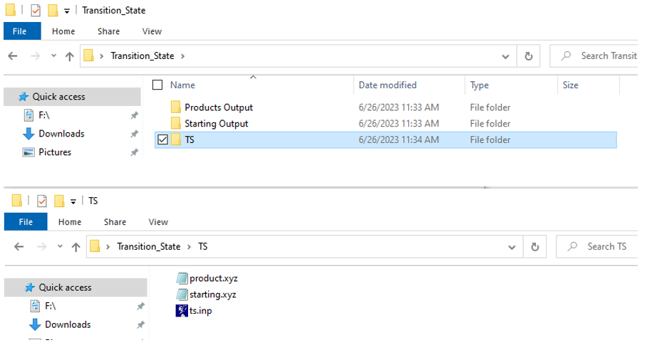
We will now walk through the calculation you need to perform to produce a reaction coordinate diagram of a simple SN2 reaction. Start by creating a folder on your desktop and name it Transition_State. After this, you should download the associated files for this computation exercise and move them to the folder that you just created. As shown in Figure 4 (top) the Transition_State Folder should contain a Starting Output, Product Output, and TS subfolder that contains the files necessary to complete the experiment. To save computational time, the energy calculations for the starting materials and products have been provided for you and can be found in the Starting Output, and Product Output file. We will be calculating the energy and structure of the transition state using Orca. As indicated above, Orca has a convenient method for finding transition states between two chemical systems. This method is referred to as nudged elastic band with transition state optimization. This method works by creating a series of “images” as intermediates between the reactants and the products of a reaction step. Each image then undergoes a constrained geometry optimization and energy calculation creating a minimal energy path between the reactants and the products. The image that is the highest in energy is then utilized to help determine the structure of the transition state.

Figure 4. The supporting files for this experiment. (Top) The complete supporting files for this exercise. (Bottom) The contents of the TS folder nested in Transition_State.

Let’s look through our input script to see what each command is doing (Figure 5). Like in previous exercises, the input script starts with a comment describing what we are trying to calculate. The second line, starting with a ! symbol, tells the computer the level of theory and basis set (B3LYP def2-SVP) as well as the calculations we want to perform (NEB-TS=Nudged Elastic Band Transition State Search, and FREQ=Frequency calculation necessary for thermochemistry data). The fourth line of the script, shown by a red arrow, indicates the ending structure to be used for the transition state search, product.xyz. The final line of the input script indicates that the starting coordinates of the structure can be found in starting.xyz. Moreover, the two numbers preceding the file name indicate the starting structure has an overall negative charge and a spin multiplicity of 1, meaning that all electrons in the structure are paired. You do not need to change any commands on this input file. The preceding description is included such that you can use this file to calculate other transition states should you desire.

Figure 5. The generic input script for determining a transition state. You do not need to change any commands within this input script. The line indicated by the red arrow shows the product of the reaction step, while the blue arrow indicates the starting materials.

We can now run our calculation using Orca via the command line as we did in the previous exercises. Briefly, open the command prompt to your PC by right clicking on the start button and searching for command prompt. First, we need to tell the computer to look on the C drive and we do this by typing C: and hitting enter. Next, we need to tell the computer where the input script and the coordinates file are to run the calculation. We do this by typing cd (space) and pasting the file path. When you hit enter the computer will paste a new line indicating that the current directory has changed, as shown in Figure 6A. To find the file path of your input script, right click on the input script (ts.inp) and select properties. The file path will appear under location, and you can highlight and copy this file path (Figure 6B).

Figure 6. (Left) Changing of the file path in the command prompt to match the location of our input script. 6B. (Right) Locating the file path on the properties window of the input script (Red Arrow).

Next, we will run the calculation by typing orca ts.inp > ts.out and pressing enter. At first it may not appear like anything is happening, but the folder on your desktop labeled TS will quickly become populated with the output of your calculation. Depending upon the speed of your computer, the calculation will take about 10-15 minutes, and upon completion the command prompt will print another line indicating that it is ready for the next command (Figure 7).

Figure 7. Running the calculation using the command line. The line indicated by the red arrow shows the computer that we want to use Orca to calculate the commands in ts.inp and that the results of this calculation should be placed in the output file ts.out. The line indicated by the blue arrow is the computer indicating that the calculation is complete, and the command prompt is ready for the next command.

Visualizing the Reaction and Transition State

You can visualize the reaction that you are modeling using some of the output files from the transition state calculation. Open the file ts_MEP _trj.xyz in Avogadro and click Extensions 🡪 Animation to bring up the window shown in Figure 8.^5,6 From here click dynamic bonds and use the slide button to move the reaction from reactants to products and back. About halfway from reactants to products will be a position where the \(\mathrm{C}-\mathrm{Cl}\) bond is partially broken and the \(\mathrm{C}-\mathrm{Br}\) bond is partially formed.

Figure 8. Examining the reaction trajectory file.

To visualize the optimized transition state please open the output file of our calculation, ts.out, in Avogadro. As shown in Figure 9 the optimized transition state shows the \(\mathrm{Br}-\mathrm{C}\) bond being formed while the \(\mathrm{C}-\mathrm{Cl}\) bond is being broken. Additionally, you will see a set of vibrational modes just like when you calculated the IR spectrum of hexane in a previous exercise. Unlike in the previous exercises, you will notice that one of the vibrational modes for this transition state will be imaginary in nature, as represented by a negative sign. Because a transition state represents the highest point on a reaction coordinate diagram there exists a vibrational mode (the imaginary mode) that if it vibrates will push the molecules either closer to products or closer to reactants. This mode will show the bonds forming and breaking at the transition states. To see this motion, click on the negative vibrational mode in the list of vibrational modes and press start animation.

Figure 9. Examining the vibrational modes of the calculated transition states. The start animation button is shown with a blue arrow.

To view the energy values associated with the transition state (calculated), or the provided reactants/products please open the respective output files in notepad. By scrolling to the end of the file you can find the total Gibbs free energy (\(G\)), as well as the enthalpy (\(H\)) and entropy (\(S\)) of the starting materials. The position of these values is shown in Figure 10 for the starting materials of our substitution reaction. Please note that entropy values are shown as \(S \times T\), \(\text{entropy} \times \text{temperature}\) in Kelvin.

Figure 10. Example output file for the starting materials of the reaction. The values for \(G\), \(H\), and \(S\) are indicated by arrows. Please note that the entropy term has already been multiplied by the temperature (298.15 K). This means that the final entropy term is really \(T \times S\).

References

1. Neese, F. The ORCA Program System. WIREs Comput. Mol. Sci. 2012, 2 (1), 73–78. https://doi.org/10.1002/wcms.81.
2. Neese, F. Software Update: The ORCA Program System, Version 4.0. WIREs Comput. Mol. Sci. 2018, 8 (1), e1327. https://doi.org/10.1002/wcms.1327.
3. Neese, F.; Wennmohs, F.; Becker, U.; Riplinger, C. The ORCA Quantum Chemistry Program Package. J. Chem. Phys. 2020, 152 (22), 224108. https://doi.org/10.1063/5.0004608.
4. Luo, Y.R. Comprehensive Handbook of Chemical Bond Energies; CRC Press: Boca Raton, FL, 2007.
5. Hanwell, M. D.; Curtis, D. E.; Lonie, D. C.; Vandermeersch, T.; Zurek, E.; Hutchison, G. R. Avogadro: An Advanced Semantic Chemical Editor, Visualization, and Analysis Platform. J. Cheminformatics 2012, 4 (1), 17. https://doi.org/10.1186/1758-2946-4-17.
6. Avogadro: An Open-Source Molecular Builder and Visualization Tool. http://avogadro.cc/.