
3.3: Computational Instructions
- Page ID
- 470361

\( \newcommand{\vecs}[1]{\overset { \scriptstyle \rightharpoonup} {\mathbf{#1}} } \)
\( \newcommand{\vecd}[1]{\overset{-\!-\!\rightharpoonup}{\vphantom{a}\smash {#1}}} \)
\( \newcommand{\id}{\mathrm{id}}\) \( \newcommand{\Span}{\mathrm{span}}\)
( \newcommand{\kernel}{\mathrm{null}\,}\) \( \newcommand{\range}{\mathrm{range}\,}\)
\( \newcommand{\RealPart}{\mathrm{Re}}\) \( \newcommand{\ImaginaryPart}{\mathrm{Im}}\)
\( \newcommand{\Argument}{\mathrm{Arg}}\) \( \newcommand{\norm}[1]{\| #1 \|}\)
\( \newcommand{\inner}[2]{\langle #1, #2 \rangle}\)
\( \newcommand{\Span}{\mathrm{span}}\)
\( \newcommand{\id}{\mathrm{id}}\)
\( \newcommand{\Span}{\mathrm{span}}\)
\( \newcommand{\kernel}{\mathrm{null}\,}\)
\( \newcommand{\range}{\mathrm{range}\,}\)
\( \newcommand{\RealPart}{\mathrm{Re}}\)
\( \newcommand{\ImaginaryPart}{\mathrm{Im}}\)
\( \newcommand{\Argument}{\mathrm{Arg}}\)
\( \newcommand{\norm}[1]{\| #1 \|}\)
\( \newcommand{\inner}[2]{\langle #1, #2 \rangle}\)
\( \newcommand{\Span}{\mathrm{span}}\) \( \newcommand{\AA}{\unicode[.8,0]{x212B}}\)
\( \newcommand{\vectorA}[1]{\vec{#1}} % arrow\)
\( \newcommand{\vectorAt}[1]{\vec{\text{#1}}} % arrow\)
\( \newcommand{\vectorB}[1]{\overset { \scriptstyle \rightharpoonup} {\mathbf{#1}} } \)
\( \newcommand{\vectorC}[1]{\textbf{#1}} \)
\( \newcommand{\vectorD}[1]{\overrightarrow{#1}} \)
\( \newcommand{\vectorDt}[1]{\overrightarrow{\text{#1}}} \)
\( \newcommand{\vectE}[1]{\overset{-\!-\!\rightharpoonup}{\vphantom{a}\smash{\mathbf {#1}}}} \)
\( \newcommand{\vecs}[1]{\overset { \scriptstyle \rightharpoonup} {\mathbf{#1}} } \)
\( \newcommand{\vecd}[1]{\overset{-\!-\!\rightharpoonup}{\vphantom{a}\smash {#1}}} \)
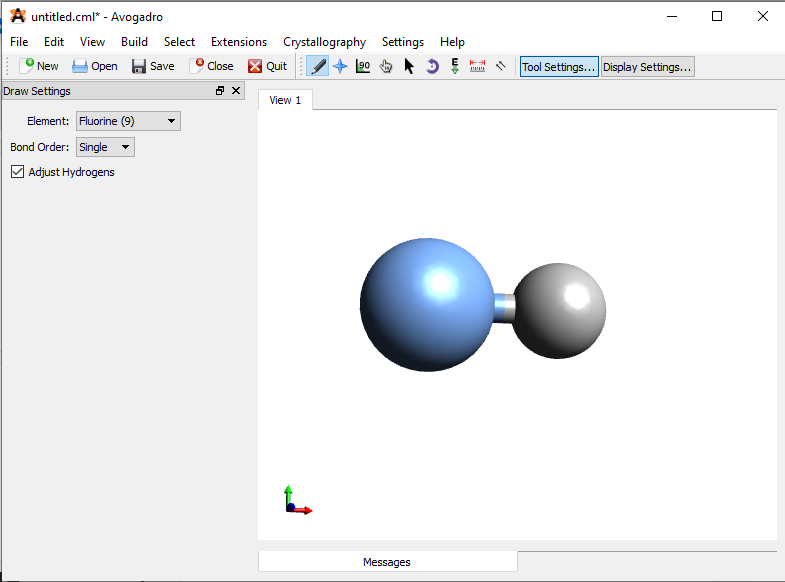
\(\newcommand{\avec}{\mathbf a}\) \(\newcommand{\bvec}{\mathbf b}\) \(\newcommand{\cvec}{\mathbf c}\) \(\newcommand{\dvec}{\mathbf d}\) \(\newcommand{\dtil}{\widetilde{\mathbf d}}\) \(\newcommand{\evec}{\mathbf e}\) \(\newcommand{\fvec}{\mathbf f}\) \(\newcommand{\nvec}{\mathbf n}\) \(\newcommand{\pvec}{\mathbf p}\) \(\newcommand{\qvec}{\mathbf q}\) \(\newcommand{\svec}{\mathbf s}\) \(\newcommand{\tvec}{\mathbf t}\) \(\newcommand{\uvec}{\mathbf u}\) \(\newcommand{\vvec}{\mathbf v}\) \(\newcommand{\wvec}{\mathbf w}\) \(\newcommand{\xvec}{\mathbf x}\) \(\newcommand{\yvec}{\mathbf y}\) \(\newcommand{\zvec}{\mathbf z}\) \(\newcommand{\rvec}{\mathbf r}\) \(\newcommand{\mvec}{\mathbf m}\) \(\newcommand{\zerovec}{\mathbf 0}\) \(\newcommand{\onevec}{\mathbf 1}\) \(\newcommand{\real}{\mathbb R}\) \(\newcommand{\twovec}[2]{\left[\begin{array}{r}#1 \\ #2 \end{array}\right]}\) \(\newcommand{\ctwovec}[2]{\left[\begin{array}{c}#1 \\ #2 \end{array}\right]}\) \(\newcommand{\threevec}[3]{\left[\begin{array}{r}#1 \\ #2 \\ #3 \end{array}\right]}\) \(\newcommand{\cthreevec}[3]{\left[\begin{array}{c}#1 \\ #2 \\ #3 \end{array}\right]}\) \(\newcommand{\fourvec}[4]{\left[\begin{array}{r}#1 \\ #2 \\ #3 \\ #4 \end{array}\right]}\) \(\newcommand{\cfourvec}[4]{\left[\begin{array}{c}#1 \\ #2 \\ #3 \\ #4 \end{array}\right]}\) \(\newcommand{\fivevec}[5]{\left[\begin{array}{r}#1 \\ #2 \\ #3 \\ #4 \\ #5 \\ \end{array}\right]}\) \(\newcommand{\cfivevec}[5]{\left[\begin{array}{c}#1 \\ #2 \\ #3 \\ #4 \\ #5 \\ \end{array}\right]}\) \(\newcommand{\mattwo}[4]{\left[\begin{array}{rr}#1 \amp #2 \\ #3 \amp #4 \\ \end{array}\right]}\) \(\newcommand{\laspan}[1]{\text{Span}\{#1\}}\) \(\newcommand{\bcal}{\cal B}\) \(\newcommand{\ccal}{\cal C}\) \(\newcommand{\scal}{\cal S}\) \(\newcommand{\wcal}{\cal W}\) \(\newcommand{\ecal}{\cal E}\) \(\newcommand{\coords}[2]{\left\{#1\right\}_{#2}}\) \(\newcommand{\gray}[1]{\color{gray}{#1}}\) \(\newcommand{\lgray}[1]{\color{lightgray}{#1}}\) \(\newcommand{\rank}{\operatorname{rank}}\) \(\newcommand{\row}{\text{Row}}\) \(\newcommand{\col}{\text{Col}}\) \(\renewcommand{\row}{\text{Row}}\) \(\newcommand{\nul}{\text{Nul}}\) \(\newcommand{\var}{\text{Var}}\) \(\newcommand{\corr}{\text{corr}}\) \(\newcommand{\len}[1]{\left|#1\right|}\) \(\newcommand{\bbar}{\overline{\bvec}}\) \(\newcommand{\bhat}{\widehat{\bvec}}\) \(\newcommand{\bperp}{\bvec^\perp}\) \(\newcommand{\xhat}{\widehat{\xvec}}\) \(\newcommand{\vhat}{\widehat{\vvec}}\) \(\newcommand{\uhat}{\widehat{\uvec}}\) \(\newcommand{\what}{\widehat{\wvec}}\) \(\newcommand{\Sighat}{\widehat{\Sigma}}\) \(\newcommand{\lt}{<}\) \(\newcommand{\gt}{>}\) \(\newcommand{\amp}{&}\) \(\definecolor{fillinmathshade}{gray}{0.9}\)Start by creating a file folder on your desktop and name it MO_Exercise. Next, you should open Avogadro on your computer and draw a molecule of hydrogen fluoride in drawing mode and minimize its energy by clicking extensions > optimize geometry. You should then save the file as HF_coord.xyz in the folder that you just created.
After creating the hydrogen fluoride coordinate file, you should download the template Orca script that we will use to tell the computer what to calculate and what coordinates to run the calculation on. Save this Orca script template as HF.inp to the MO Exercise folder that you created above.
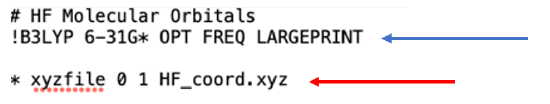
As was the case with the previous exercise, the Orca script template, shown in Figure 3, starts with a # symbol which indicates a comment line where we can describe the calculation that we are performing. The second line, which begins with a ! symbol, tells Orca the functional of the calculation (B3LYP), the basis set (6-31G*), and what we are asking the program to calculate (OPT-geometry optimization, FREQ-thermodynamic properties calculation). On line 4, which begins with a * symbol, you tell Orca what file contains the coordinate files for our molecule(s). The phrase xyzfile tells the computer that the file you are using has the molecule in XYZ cartesian coordinates. There are then a series of two numbers which provide information about charge and spin of the reaction. The first number is the total net charge of molecule(s) in the XYZ file, in this case it is zero because HF is a neutral molecule. The second number is the net spin multiplicity (S) of the molecule that you are calculating, which in this case is 1 (singlet) indicating that all electrons in the molecule are paired.
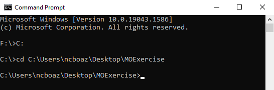
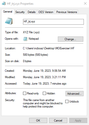
We can now run our calculation using Orca via the command line as we did in the previous exercise. Briefly, open the command prompt to your PC by right clicking on the start button and searching for command prompt. First, we need to tell the computer to look on the C drive and we do this by typing C: in the command prompt and hitting enter. Next, we need to tell the computer where the input script and the coordinates file are to run the calculation. We do this by typing cd (space) and pasting the file path into the command prompt. When you hit enter the computer will paste a new line indicating that the current directory has changed, as shown in Figure 4A. To find the file path of your input script, right click on the input script (HF.inp) and select properties. The file path will appear under location, and you can highlight and copy this file path (Figure 4 B).
Next, we will run the calculation by typing orca HF.inp > HF.out and pressing enter in the command prompt. At first, it may not appear like anything is happening but the folder on your desktop housing the input file will quickly become populated with the output of your calculation. Depending upon the speed of your computer the calculation will take from 1-5 minutes, and upon completion the command prompt will print another line indicating that it is ready for the next command (Figure 5).

Examining Calculated Molecular Orbitals
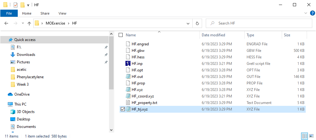
Upon completion of the calculation, Orca will deposit a series of files in your working folder as shown in Figure 6. The file containing the molecular orbitals that we calculated from HF is the HF.out file.
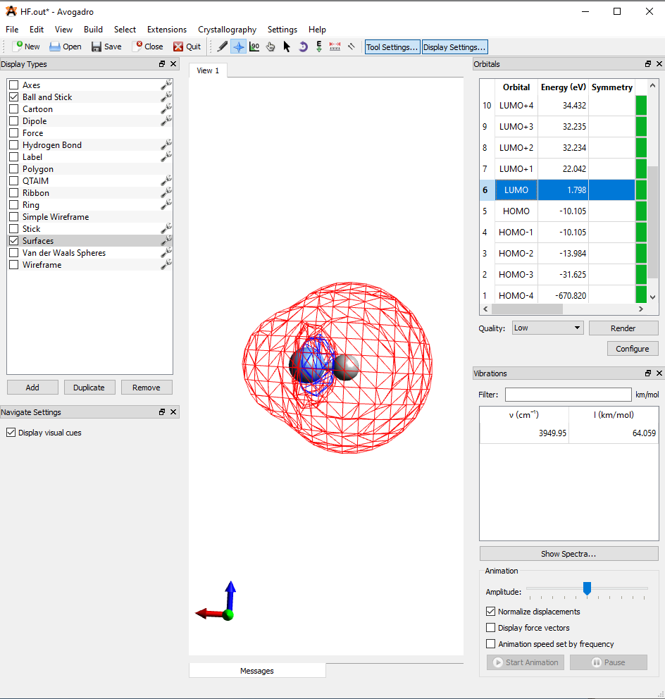
To view the molecular orbitals of HF you will first need to open the output file HF.out from your calculation in Avogadro. As shown in Figure 7, the HF.out file will show the molecular orbitals in the upper right portion of the screen.

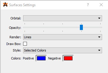
Before you view any of the molecular orbitals you will need to click on the wrench button adjacent to the surfaces option link (See Figure 7). This will bring up a panel where you can change the positive and negative surfaces to blue and red respectively as shown in Figure 8. Also, to make the orbitals easier to see you should change the background color by clicking View > Set Background Color > White.
By clicking on any of the molecular orbitals in the upper right, you can visualize what these molecular orbitals will look like as well as see the energy levels of these orbitals (Figure 9). H.O.M.O-3 to LUMO represent the molecular orbitals shown in Figure 1. H.O.M.O-4 represents the \(1S\) orbital of the fluorine atom. You will notice that the molecular orbitals don’t look exactly like the versions of the molecular orbitals that we approximated by overlapping the hybrid orbitals of fluorine in and out of phase with the 1s orbital of hydrogen. The reason for this is that when molecular orbitals are constructed using a computer, non-hybridized atomic orbitals are directly used in the linear combination of orbitals to construct molecular orbitals. Moreover, Orca is going to compute these orbitals mathematically instead of just visually. Now that you’ve completed the computational exercise, please answer the questions at the end of this assignment.
References
- Neese, F. Software Update: The ORCA Program System, Version 4.0. WIREs Comput. Mol. Sci. 2018, 8 (1), e1327. https://doi.org/10.1002/wcms.1327.
- Neese, F. The ORCA Program System. WIREs Comput. Mol. Sci. 2012, 2 (1), 73–78. https://doi.org/10.1002/wcms.81.
- Neese, F.; Wennmohs, F.; Becker, U.; Riplinger, C. The ORCA Quantum Chemistry Program Package. J. Chem. Phys. 2020, 152 (22), 224108. https://doi.org/10.1063/5.0004608.
- Hanwell, M. D.; Curtis, D. E.; Lonie, D. C.; Vandermeersch, T.; Zurek, E.; Hutchison, G. R. Avogadro: An Advanced Semantic Chemical Editor, Visualization, and Analysis Platform. J. Cheminformatics 2012, 4 (1), 17. https://doi.org/10.1186/1758-2946-4-17.
- Avogadro: An Open-Source Molecular Builder and Visualization Tool.