LS8. Solutions to Selected Problems
- Page ID
- 4297
\( \newcommand{\vecs}[1]{\overset { \scriptstyle \rightharpoonup} {\mathbf{#1}} } \)
\( \newcommand{\vecd}[1]{\overset{-\!-\!\rightharpoonup}{\vphantom{a}\smash {#1}}} \)
\( \newcommand{\id}{\mathrm{id}}\) \( \newcommand{\Span}{\mathrm{span}}\)
( \newcommand{\kernel}{\mathrm{null}\,}\) \( \newcommand{\range}{\mathrm{range}\,}\)
\( \newcommand{\RealPart}{\mathrm{Re}}\) \( \newcommand{\ImaginaryPart}{\mathrm{Im}}\)
\( \newcommand{\Argument}{\mathrm{Arg}}\) \( \newcommand{\norm}[1]{\| #1 \|}\)
\( \newcommand{\inner}[2]{\langle #1, #2 \rangle}\)
\( \newcommand{\Span}{\mathrm{span}}\)
\( \newcommand{\id}{\mathrm{id}}\)
\( \newcommand{\Span}{\mathrm{span}}\)
\( \newcommand{\kernel}{\mathrm{null}\,}\)
\( \newcommand{\range}{\mathrm{range}\,}\)
\( \newcommand{\RealPart}{\mathrm{Re}}\)
\( \newcommand{\ImaginaryPart}{\mathrm{Im}}\)
\( \newcommand{\Argument}{\mathrm{Arg}}\)
\( \newcommand{\norm}[1]{\| #1 \|}\)
\( \newcommand{\inner}[2]{\langle #1, #2 \rangle}\)
\( \newcommand{\Span}{\mathrm{span}}\) \( \newcommand{\AA}{\unicode[.8,0]{x212B}}\)
\( \newcommand{\vectorA}[1]{\vec{#1}} % arrow\)
\( \newcommand{\vectorAt}[1]{\vec{\text{#1}}} % arrow\)
\( \newcommand{\vectorB}[1]{\overset { \scriptstyle \rightharpoonup} {\mathbf{#1}} } \)
\( \newcommand{\vectorC}[1]{\textbf{#1}} \)
\( \newcommand{\vectorD}[1]{\overrightarrow{#1}} \)
\( \newcommand{\vectorDt}[1]{\overrightarrow{\text{#1}}} \)
\( \newcommand{\vectE}[1]{\overset{-\!-\!\rightharpoonup}{\vphantom{a}\smash{\mathbf {#1}}}} \)
\( \newcommand{\vecs}[1]{\overset { \scriptstyle \rightharpoonup} {\mathbf{#1}} } \)
\( \newcommand{\vecd}[1]{\overset{-\!-\!\rightharpoonup}{\vphantom{a}\smash {#1}}} \)
\(\newcommand{\avec}{\mathbf a}\) \(\newcommand{\bvec}{\mathbf b}\) \(\newcommand{\cvec}{\mathbf c}\) \(\newcommand{\dvec}{\mathbf d}\) \(\newcommand{\dtil}{\widetilde{\mathbf d}}\) \(\newcommand{\evec}{\mathbf e}\) \(\newcommand{\fvec}{\mathbf f}\) \(\newcommand{\nvec}{\mathbf n}\) \(\newcommand{\pvec}{\mathbf p}\) \(\newcommand{\qvec}{\mathbf q}\) \(\newcommand{\svec}{\mathbf s}\) \(\newcommand{\tvec}{\mathbf t}\) \(\newcommand{\uvec}{\mathbf u}\) \(\newcommand{\vvec}{\mathbf v}\) \(\newcommand{\wvec}{\mathbf w}\) \(\newcommand{\xvec}{\mathbf x}\) \(\newcommand{\yvec}{\mathbf y}\) \(\newcommand{\zvec}{\mathbf z}\) \(\newcommand{\rvec}{\mathbf r}\) \(\newcommand{\mvec}{\mathbf m}\) \(\newcommand{\zerovec}{\mathbf 0}\) \(\newcommand{\onevec}{\mathbf 1}\) \(\newcommand{\real}{\mathbb R}\) \(\newcommand{\twovec}[2]{\left[\begin{array}{r}#1 \\ #2 \end{array}\right]}\) \(\newcommand{\ctwovec}[2]{\left[\begin{array}{c}#1 \\ #2 \end{array}\right]}\) \(\newcommand{\threevec}[3]{\left[\begin{array}{r}#1 \\ #2 \\ #3 \end{array}\right]}\) \(\newcommand{\cthreevec}[3]{\left[\begin{array}{c}#1 \\ #2 \\ #3 \end{array}\right]}\) \(\newcommand{\fourvec}[4]{\left[\begin{array}{r}#1 \\ #2 \\ #3 \\ #4 \end{array}\right]}\) \(\newcommand{\cfourvec}[4]{\left[\begin{array}{c}#1 \\ #2 \\ #3 \\ #4 \end{array}\right]}\) \(\newcommand{\fivevec}[5]{\left[\begin{array}{r}#1 \\ #2 \\ #3 \\ #4 \\ #5 \\ \end{array}\right]}\) \(\newcommand{\cfivevec}[5]{\left[\begin{array}{c}#1 \\ #2 \\ #3 \\ #4 \\ #5 \\ \end{array}\right]}\) \(\newcommand{\mattwo}[4]{\left[\begin{array}{rr}#1 \amp #2 \\ #3 \amp #4 \\ \end{array}\right]}\) \(\newcommand{\laspan}[1]{\text{Span}\{#1\}}\) \(\newcommand{\bcal}{\cal B}\) \(\newcommand{\ccal}{\cal C}\) \(\newcommand{\scal}{\cal S}\) \(\newcommand{\wcal}{\cal W}\) \(\newcommand{\ecal}{\cal E}\) \(\newcommand{\coords}[2]{\left\{#1\right\}_{#2}}\) \(\newcommand{\gray}[1]{\color{gray}{#1}}\) \(\newcommand{\lgray}[1]{\color{lightgray}{#1}}\) \(\newcommand{\rank}{\operatorname{rank}}\) \(\newcommand{\row}{\text{Row}}\) \(\newcommand{\col}{\text{Col}}\) \(\renewcommand{\row}{\text{Row}}\) \(\newcommand{\nul}{\text{Nul}}\) \(\newcommand{\var}{\text{Var}}\) \(\newcommand{\corr}{\text{corr}}\) \(\newcommand{\len}[1]{\left|#1\right|}\) \(\newcommand{\bbar}{\overline{\bvec}}\) \(\newcommand{\bhat}{\widehat{\bvec}}\) \(\newcommand{\bperp}{\bvec^\perp}\) \(\newcommand{\xhat}{\widehat{\xvec}}\) \(\newcommand{\vhat}{\widehat{\vvec}}\) \(\newcommand{\uhat}{\widehat{\uvec}}\) \(\newcommand{\what}{\widehat{\wvec}}\) \(\newcommand{\Sighat}{\widehat{\Sigma}}\) \(\newcommand{\lt}{<}\) \(\newcommand{\gt}{>}\) \(\newcommand{\amp}{&}\) \(\definecolor{fillinmathshade}{gray}{0.9}\)Problem LS1.1.
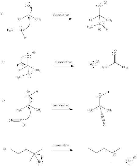
- a bromine atom replaces a hydrogen atom
- an acetate group (ethanoyl ester) replaces a bromine atom
- a bromine atom replaces a chlorine atom (or ions)
- a methoxy group replaces a chlorine atom
- a methylamino group replaces an oxygen atom
Problem LS2.1.
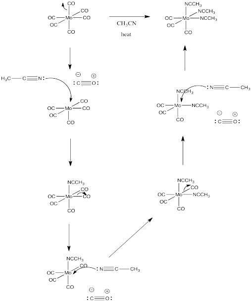
- Energy is released when bonds are formed. Energy must be added to break bonds. In general, bond-breaking costs more energy than bond-making.
- On the basis of question (a), we would assume that the second, bond-breaking step is the rate determining step in association mechanisms.
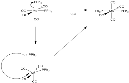
- The first, dissociative step would be the rate-determining step, on the basis of question (a).
- The rate law would include steps prior t the rate determining step. Rate = k[MLn][X] if MLn is the complex and X is the new ligand.
- Rate = k[MLn].
Problem LS2.5.
This problem is answered through consideration of the spectrochemical series.
from easiest to hardest to replace: NO3- Cl- H2O NH3 PPh3 CO
Problem LS3.1.
Associative Rate Law: Rate = [MLn][X], if MLn is the complex and X is the new ligand.
- Rate will quadruple: Rate = (2 x [MLn]0) x (2 x [X]0) = 4 x [MLn]0[X]0, if [X]0 and [MLn]0 are the original concentrations.
- Rate will sextuple: Rate = (3 x [MLn]0) x (2 x [X]0) = 6 x [MLn]0[X]0.
- Rate will nonuple: Rate = (3 x [MLn]0) x (3 x [X]0) = 9 x [MLn]0[X]0.
- Rate will stay the same: Rate = (0.5 x [MLn]0) x (2 x [X]0) = 1 x [MLn]0[X]0.
Problem LS3.3.
- Changing both concentrations at once would leave some doubt about whether one concentration had affected the rate, or the other concentration, or both. In practice, one concentration is usually held constant while the other is kept in excess and varied.
- Rate changes over time because the concentrations of reactants change as they are consumed. By reporting only the initial rate (usually meaning less than 5% or 10% complete, but possibly even less than that if a lot of data can be gathered very quickly), the concentrations are still about what you started with. That means you can report a rate that corresponds to a given concentration with confidence.
Problem LS3.4.
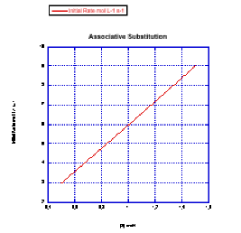
- The rate would change with the ligand concentration if associative. This rate is constant over a range of ligand concentrations, so the reaction is not associative.
- The rate increases linearly with ligand concentration. This reaction proceeds via an associative mechanism.
- The rate changes over the concentration range, but it decreases. This is the opposite of what should happen. This reaction does not follow a simple associative pathway.
- The rate increases linearly with ligand concentration. This reaction proceeds via an associative mechanism.
Problem LS3.5.
Because Rate = k[MLn][L] and [MLn] is held constant while [L] is varied, then the slope of the line is k [MLn]. Since you would know the value of [MLn], you could obtain the rate constant from the quantity (slope/ [MLn]).
Problem LS4.1.
- 4 minutes = 240 seconds = 2 x 120 second = 2 half lives. Material left = 50% x 50% = 0.5 x 0.5 = 0.25 = 25% left
- 6 minutes = 360 seconds = 3 x 120 second = 3 half lives. Material left = 0.5 x 0.5 x 0.5 = 0.125 = 12.5% left
- 8 minutes = 480 seconds = 4 x 120 second = 4 half lives. Material left = 0.5 x 0.5 x 0.5 x 0.5 = 0.0625 = 6.25% left
- 10 minutes = 600 seconds = 5 x 120 second = 5 half lives. Material left = 0.5 x 0.5 x 0.5 x 0.5 x 0.5 = 0.03125 = 3.125% left
Problem LS4.2.
Dissociative Rate Law: Rate = [MLn], if MLn is the complex. There is no dependence on [X], if X is the new ligand.
- Rate will double: Rate = 2 x [MLn]0, if [MLn]0 is the original concentration.
- Rate will triple: Rate = 3 x [MLn]0.
- Rate will triple: Rate = 3 x [MLn]0.
- Rate will be halved: Rate = 0.5 x [MLn]0.
Problem LS4.4.
- The rate increases with both concentration of metal complex and incoming ligand. This looks like an associative mechanism.
- The rate depends on concentration of the metal complex, but not the incoming ligand. This looks like a dissociative mechanism.
- The rate depends on the concentration of incoming ligand, but not the metal complex. Whatever is going on here, it isn't a simple dissociative mechanism.
Problem LS4.5.
- The rate of the reaction is depressed when the concentration of the departing ligand is increased.
- This dependence could indicate an equilibrium in the dissociative step. The more departing ligand is added, the more the equilibrium is pushed back towards the original metal complex. With less dissociated metal complex around, the entering ligand cannot form the new complex as quickly.
Problem LS4.6.
- These solvents all have lone pairs. They could be Lewis bases or nucleophiles.
- It looks like two competing mechanisms. On term suggests a dissociative mechanism, whereas the other term suggests a dissociative mechanism. They could be happening in competition with each other.
- On the other hand, it could be that there is one mechanism with two different nucleophiles. If the incoming ligand is the nucleophile, the term on the right shows up in the rate law. If the solvent is the nucleophile, forming a third complex, the term on the left shows up in the rate law. That's because we would typically change the amount of metal complex and the amount of ligand that we add to the solution in order to determine the rate law, but we wouldn't normally be able to change the concentration of the solvent, so it would be a constant. (How could you confirm this explanation in an experiment?)
Problem LS5.2.
The metal centre is becoming more crowded as the new ligand arrives, so an increase in energy owing to steric hindrance may also play a role in the transition state energetics.
Problem LS5.3.
a) The new ligand, B, is arriving at the same time as the old ligand, A, is departing. We might also describe it as new ligand B pushing old ligand A out of the complex.
b) Rate = k[ML5A][B], which looks like an associative rate law.
c) This is a thought-provoking question without a definite answer. Associative mechanisms typically have lower activation enthalpy than dissociative mechanisms, because there has also been some bond-making prior to the bond-breaking in the rate determining step. The associative interchange would be a little more like the associative mechanism than dissociative. The mix of bond-making and bond-breaking at the transition state would make the enthalpy of activation relatively low.
Associative mechanisms have negative activation entropies, whereas dissociative mechanisms have positive activation entropies. The associative interchange could be in between the two, given that the elementary step would be close to entropically neutral overall. What happens at the transition state is a little harder to imagine, but it might reflect the small changes in entropy through the course of the reaction, producing a small entropy of activation. On the other hand, if the incoming ligand is forced to adopt some specific approach as it comes into the molecule (to stay out of the way of the departing ligand, for example) then that restriction could show up as a small negative activation entropy.
Problem LS5.4.
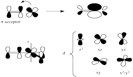
a) The lone pair donation from one ligand appears to push another ligand out.
b) The first step is probably rate determining, because of the bond breaking involved.
c) If the first step is rate determining, Rate = k [ML5A].
d) Another question without a very clear answer. Compared with an associative mechanism, the activation entropy is probably much more positive, because additional degrees of freedom are being gained as the molecule heads over the activation barrier and one of the ligands separates to be on its own. However, the activation entropy may be less positive than in a regular dissociation, because in this case the breaking of one bond has to be coordinated with the formation of another.
The enthalpy of activation has both a bond-making and bond-breaking component, a little like in an associative mechanism. However, the amount of bond making here is probably less important, because pi bonds are typically not as strong as sigma bonds. The activation enthalpy is probably higher than an associative pathway but not as high as a dissociative one.
e) The donor ligand must have a lone pair. Oxygen donors would be good candidates, because even if one lone pair is already donating in a sigma bond, an additional lone pair may be available for pi donation. The same thing is true for halogen donors. It would also be true for anionic nitrogen donors but not for neutral nitrogen donors, because a neutral nitrogen has only one lone pair.
Problem LS7.1.
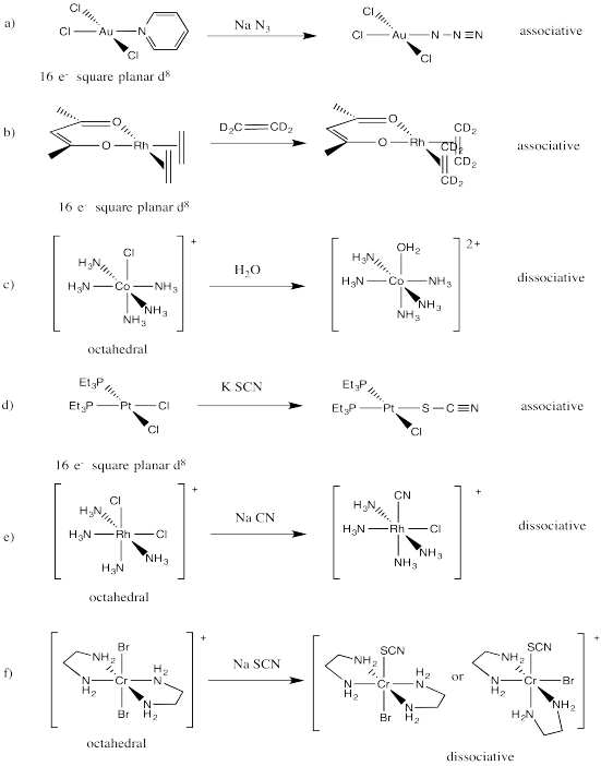
This is probably an associative mechanism because of the square planar geometry.
Problem LS7.4.
There is an electronegativity trend: the less electronegative, the greater the trans effect (see the halogens, as well as the series O,N,C and also the orders within several pairings: S,P; O,S and N,P).
Alternatively, some of the above could be described by a polarizability trend: more polarizable atom, greater trans effect (for example, the halogens).
Most of the ligands containing π-bonds have strong trans influence (but not all).
Most of the π-donors have a weaker trans influence. However, these ligand cover a very broad range in this series.
Problem LS7.5.
The strongest σ-donors are typically those with more polarizable donor atoms (such as S, P, I) as well as those with less electronegative donor ions such as C- and H-.


