6.3: Characteristics of C-13 NMR Spectroscopy

Learning Objectives

• Understand where different types of carbon appear on the spectrum

Simply, ¹³C NMR allows you to determine how many different carbons are in a molecule. It will also be seen that information on functional groups present in a molecule can be determined using ¹³C NMR. In a spectrum, each signal represents a resonance for a different carbon atom. The typical range for the resonance frequencies is 0 to 220 ppm from tetramethylsilane (TMS) reference. Like ¹H NMR, the chemical shift of ¹³C nuclei is influenced by its chemical environment like the ¹H nuclei. 

One of the greatest advantages of ¹³C-NMR compared to ¹H-NMR is the breadth of the spectrum - carbons resonate from 0-220 ppm relative to the TMS standard, as opposed to only 0-12 ppm for protons. Because of this, ¹³C signals rarely overlap, meaning we can almost always distinguish separate peaks for each carbon, even in a relatively large compound containing carbons in very similar environments. In a ¹H NMR spectrum of 1-heptanol, for example, many of the signals overlap and it becomes difficult to analyze, only the signals for the alcohol proton (H_a) and the two protons on the adjacent carbon (H_b) are easily analyzed.

In the ¹³C spectrum of 1-heptanol, we can easily distinguish each carbon signal, and we know from this data that our sample has seven non-equivalent carbons. (Notice also that, as we would expect, the chemical shifts of the carbons get progressively smaller as they get farther away from the deshielding oxygen.)

This property of ¹³C NMR makes it very helpful in the elucidation of larger, more complex structures.

Example \(\PageIndex{1}\)

Predict the number of carbon resonances expected in a ¹³C NMR spectrum of ethyl prop-2-enoate, C₅H₈O₂. 

Solution

There is no symmetry in this molecule, so you would expect 5 resonances - one for each C in the molecule - in a ¹³C NMR spectrum.

¹³C NMR spectrum of ethyl prop-2-en-oate:

¹³C NMR Chemical Shifts

The ¹³C NMR is used for determining functional groups based on characteristic shift values. ¹³C chemical shifts are greatly affected by electronegative effects and magnetic anisotropy. If a H atom in an alkane is replaced by substituent X, electronegative atoms (O, N, halogen), ¹³C signals for nearby carbons shift downfield (left; increase in ppm) with the effect diminishing with distance from the electron withdrawing group just as in ¹H NMR. Below, a typical ¹³C chemical shift table shows the regions of some of the common organic functional groups.

 

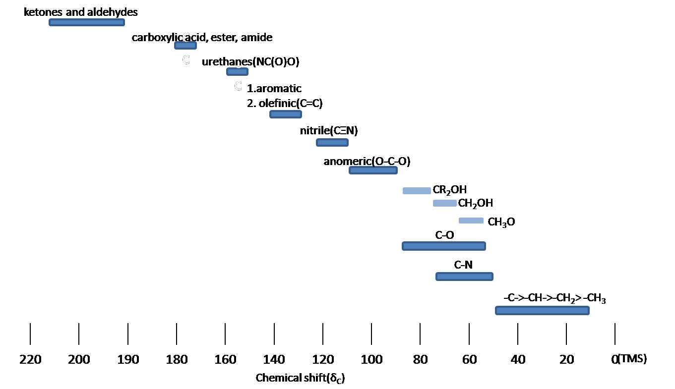
 ¹³C Chemical shift range for organic compounds

 

Example \(\PageIndex{2}\)

Assign the resonances in a ¹³C NMR spectrum of ethyl prop-2-enoate, C₅H₈O₂.

Solution

There are 5 carbons in the molecule, which equate to the 5 peaks in the ¹³C NMR spectrum. 

Exercise \(\PageIndex{1}\)

Using ¹³C NMR spectrum, how could you tell the difference between the isomers acetone and methoxy ethene? 

 vs. 

 

Answer

There are a few ways to tell the difference between the two molecules. Acetone would have 2 different resonances in a ¹³C NMR spectrum due to the symmetry of the molecule. Acetone is a ketone and ketone carbons appear far downfield 180-220 ppm. Methoxy ethene is difunctional molecule with an ether and an alkene. It would show 3 resonances in the ¹³C NMR spectrum, which all would be lower than the ketone resonance. Alkene resonances are 100-150 ppm and a C-O bond would be 40-85 ppm. 

Exercise \(\PageIndex{2}\)

Assign as many peaks as you can to the 13C NMR spectrum to specific carbons in the N-ethylbenzamide. 

  

¹³C NMR spectrum: 

Answer

While there are 9 total carbons, there are only 7 non-equivalent carbons.

Labeled Carbon Number	Chemical Shift (ppm)
1	14.80
2	34.80
3	134.40
4	126.70
5	128.10
6	130.90
7	167.20

 

 

Contributors and Attributions

• Prof. Steven Farmer (Sonoma State University)

• Organic Chemistry With a Biological Emphasis by Tim Soderberg (University of Minnesota, Morris)

• Chris P Schaller, Ph.D., (College of Saint Benedict / Saint John's University)