2.2: Introduction to reaction kinetics- Basic rate laws

The kinetic theory of gases can be used to model the frequency of collisions between hard-sphere molecules, which is proportional to the reaction rate. Most systems undergoing a chemical reaction, however, are much more complex. The reaction rates may be dependent on specific interactions between reactant molecules, the phase(s) in which the reaction takes place, etc. The field of chemical kinetics is thus by-and-large based on empirical observations. From experimental observations, scientists have established that reaction rates almost always have a power-law dependence on the concentrations of one or more of the reactants. In the following sections, we will discuss different power laws that are commonly observed in chemical reactions.

\(0^{th}\) Order Reaction Kinetics

Consider a closed container initially filled with chemical species \(A\). At \(t = 0\), a stimulus, such as a change in temperature, the addition of a catalyst, or irradiation, causes an irreversible chemical reaction to occur in which \(A\) transforms into product \(B\):

\[a \text{A} \longrightarrow b \text{B}\]

The rate that the reaction proceeds, \(r\), can be described as the change in the concentrations of the chemical species with respect to time:

\[r = -\dfrac{1}{a} \dfrac{d \left[ \text{A} \right]}{dt} = \dfrac{1}{b} \dfrac{d \left[ \text{B} \right]}{dt} \label{19.1}\]

where \(\left[ \text{X} \right]\) denotes the molar concentration of chemical species \(\text{X}\) with units of \(\frac{\text{mol}}{\text{L}^3}\).

Let us first examine a reaction \(\text{A} \longrightarrow \text{B}\) in which the reaction rate, \(r\), is constant with time:

\[r = -\dfrac{d \left[ \text{A} \right]}{dt} = k \label{19.2}\]

where \(k\) is a constant, also known as the rate constant with units of \(\dfrac{\text{mol}}{\text{m}^3 \text{s}}\). Such reactions are called zeroth order reactions because the reaction rate depends on the concentrations of species \(\text{A}\) and \(\text{B}\) to the \(0^{th}\) power. Integrating \(\left[ \text{A} \right]\) with respect to \(T\), we find that

\[\left[ \text{A} \right] = -kt + c_1 \label{19.3}\]

At \(t = 0\), \(\left[ \text{A} \right] \left( 0 \right) = \left[ \text{A} \right]_0\). Plugging these values into the equation, we find that \(c_1 = \left[ \text{A} \right]_0\). The final form of the equation is:

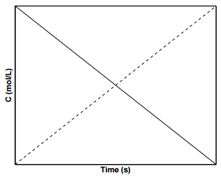
\[\left[ \text{A} \right] = \left[ \text{A} \right]_0 - kt \label{19.4}\]

A plot of the concentration of species \(\text{A}\) with time for a \(0^{th}\) order reaction is shown in Figure \(\PageIndex{1}\), where the slope of the line is \(-k\) and the \(y\)-intercept is \(\left[ \text{A} \right]_0\). Such reactions in which the reaction rates are independent of the concentrations of products and reactants are rare in nature. An example of a system displaying \(0^{th}\) order kinetics would be one in which a reaction is mediated by a catalyst present in small amounts.

\(1^{st}\) Order Reaction Kinetics

Experimentally, it is observed than when a chemical reaction is of the form

\[\sum_i \nu_i \text{A}_i = 0 \label{19.5}\]

the reaction rate can be expressed as

\[ r = k \prod_\text{reactants} \left[ \text{A}_i \right]^{\nu_i} \label{19.6}\]

where it is assumed that the stoichiometric coefficients \(\nu_i\) of the reactants are all positive. Thus, or a reaction \(\text{A} \longrightarrow \text{B}\), the reaction rate depends on \(\left[ \text{A} \right]\) raised to the first power:

\[r = \dfrac{d \left[ \text{A} \right]}{dt} = -k \left[ \text{A} \right] \label{19.7}\]

Figure \(\PageIndex{1}\): Plots of \(\left[ \text{A} \right]\) (solid line) and \(\left[ \text{B} \right]\) (dashed line) over time for a \(0^{th}\) order reaction.

For first order reactions, \(k\) has the units of \(\dfrac{1}{\text{s}}\). Integrating and applying the condition that at \(t = 0 \: \text{s}\), \(\left[ \text{A} \right] = \left[ \text{A} \right]_0\), we arrive at the following equation:

\[\left[ \text{A} \right] = \left[ \text{A} \right] e^{-kt} \label{19.8}\]

Figure \(\PageIndex{2}\) displays the concentration profiles for species \(\text{A}\) and \(\text{B}\) for a first order reaction. To determine the value of \(k\) from

Figure \(\PageIndex{2}\): Plots of \(\left[ \text{A} \right]\) (solid line) and \(\left[ \text{B} \right]\) (dashed line) over time for a \(1^{st}\) order reaction.

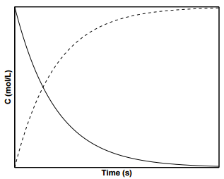
experimental data, it is convenient to take the natural log of Equation 19.8:

\[\text{ln} \left( \left[ \text{A} \right] \right) = \text{ln} \left( \left[ \text{A} \right]_0 \right) - kt \label{19.9}\]

For a first order irreversible reaction, a plot of \(\text{ln} \left( \left[ \text{A} \right] \right)\) vs. \(t\) is straight line with a slope of \(-k\) and a \(y\)-intercept of \(\text{ln} \left( \left[ \text{A} \right]_0 \right)\).

\(2^{nd}\) Order Reaction Kinetics

Another type of reaction depends on the square of the concentration of species \(\text{A}\) - these are known as second order reactions. For a second order reaction in which \(2 \text{A} \longrightarrow \text{B}\), we can write the reaction rate to be

\[r = -\dfrac{1}{2} \dfrac{d \left[ \text{A} \right]}{dt} = k \left[ \text{A} \right]^2 \label{19.10}\]

For second order reactions, \(k\) has the units of \(\dfrac{\text{m}^3}{\text{mol} \cdot \text{s}}\). Integrating and applying the condition that at \(t = 0 \: \text{s}\), \(\left[ \text{A} \right] = \left[ \text{A} \right]_0\), we arrive at the following equation for the concentration of \(\text{A}\) over time:

\[\left[ \text{A} \right] = \dfrac{1}{2kt + \dfrac{1}{\left[ \text{A} \right]_0}} \label{19.11}\]

Figure \(\PageIndex{3}\) shows concentration profiles of \(\text{A}\) and \(\text{B}\) for a second order reaction. To determine \(k\) from experimental data for

Figure \(\PageIndex{3}\): Plots of \(\left[ \text{A} \right]\) (solid line) and \(\left[ \text{B} \right]\) (dashed line) over time for a \(2^{nd}\) order reaction.

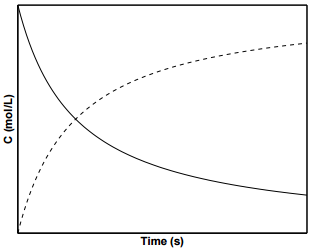
second-order reactions, it is convenient to invert Equation 19.11:

\[\dfrac{1}{\left[ \text{A} \right]} = \dfrac{1}{\left[ \text{A} \right]_0} + 2kt \label{19.12}\]

A plot of \(1/\left[ \text{A} \right]\) vs. \(t\) will give rise to a straight line with slope \(k\) and intercept \(1/\left[ \text{A} \right]_0\).

Second order reaction rates can also apply to reactions in which two species react with each other to form a product:

\[\text{A} + \text{B} \overset{k}{\longrightarrow} \text{C}\]

In this scenario, the reaction rate will depend on the concentrations of both \(\text{A}\) and \(\text{B}\) to the first order:

\[r = -\dfrac{d \left[ \text{A} \right]}{dt} = -\dfrac{d \left[ \text{B} \right]}{dt} = k \left[ \text{A} \right] \left[ \text{B} \right] \label{19.13}\]

In order to integrate the above equation, we need to write it in terms of one variable. Since the concentrations of \(\text{A}\) and \(\text{B}\) are related to each other via the chemical reaction equation, we can write:

\[\left[ \text{B} \right] = \left[ \text{B} \right]_0 - \left( \left[ \text{A} \right]_0 - \left[ \text{A} \right] \right) = \left[ \text{A} \right] + \left[ \text{B} \right]_0 - \left[ \text{A} \right]_0 \label{19.14}\]

\[\dfrac{d \left[ \text{A} \right]}{dt} = -k \left[ \text{A} \right] \left( \left[ \text{A} \right] + \left[ \text{B} \right]_0 - \left[ \text{A} \right]_0 \right) \label{19.15}\]

We can then use partial fractions to integrate:

\[kdt = \dfrac{d \left[ \text{A} \right]}{\left[ \text{A} \right] \left( \left[ \text{A} \right] + \left[ \text{B} \right]_0 - \left[ \text{A} \right]_0 \right)} = \dfrac{1}{\left[ \text{B} \right]_0 - \left[ \text{A} \right]_0} \left( \dfrac{d \left[ \text{A} \right]}{\left[ \text{A} \right]} - \dfrac{d \left[ \text{A} \right]}{\left[ \text{B} \right]_0 - \left[ \text{A} \right]_0 + \left[ \text{A} \right]} \right) \label{19.16}\]

\[kt = \dfrac{1}{\left[ \text{A} \right]_0 - \left[ \text{B} \right]_0} \text{ln} \dfrac{\left[ \text{A} \right] \left[ \text{B} \right]_0}{\left[ \text{B} \right] \left[ \text{A} \right]_0} \label{19.17}\]

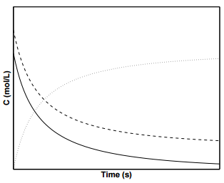
Figure \(\PageIndex{4}\) displays the concentration profiles of species \(\text{A}\), \(\text{B}\), and \(\text{C}\) for a second order reaction in which the initial concentrations of \(\text{A}\) and \(\text{B}\) are not equal.

Rate Laws for Elementary Reactions

In general, it is necessary to experimentally measure the concentrations of species over time in order to determine the apparent rate law governing the reaction. If the reactions are elementary reactions, (i.e. they cannot be expressed as a series of simpler reactions), then we can directly define the rate law based on the chemical equation. For example, an elementary

Figure \(\PageIndex{4}\): Plots of \(\left[ \text{A} \right]\) (solid line), \(\left[ \text{B} \right]\) (dashed line) and \(\left[ \text{C} \right]\) (dotted line) over time for a \(2^{nd}\) order reaction in which the initial concentrations of the reactants, \(\left[ \text{A} \right]_0\) and \(\left[ \text{B} \right]_0\), are not equal.

reaction in which a single reactant transforms into a single product, is unimolecular reaction. These reactions follow \(1^{st}\) order rate kinetics. An example of this type of reaction would be the isomerization of butane:

\[nC_4 H_{10} \longrightarrow iC_4 H_{10}\]

From the chemical reaction equation, we can directly write the rate law as

\[\dfrac{d \left[ nC_4 H_{10} \right]}{dt} = -k \left[ nC_4 H_{10} \right] \label{19.18}\]

without the need to carry out experiments.

Elementary bimolecular reactions that involve two molecules interacting to form one or more products follow second order rate kinetics. An example would be the following reaction between a nitrate molecule and carbon monoxide to form nitrogen dioxide and carbon dioxide:

\[NO_3 + CO \longrightarrow NO_2 + CO_2\]

For the above elementary reaction, we can directly write the rate law as:

\[\dfrac{d \left[ NO_3 \right]}{dt} = -k \left[ NO_3 \right] \left[ CO \right] \label{19.19}\]

Trimolecular elementary reactions involving three reactant molecules to form one or more products are rare due to the low probability of three molecules simultaneously colliding with one another.

Reversible Reactions

Oftentimes, reactions are reversible, meaning that a reaction can proceed in both directions. An example of a reversible reaction is the isomerization of cis-\(1\),\(2\)-dichloroethene to trans-\(1\),\(2\)-dichloroethene. At equilibrium, both isomers are present, with their equilibrium concentrations determined by the rate at which the forward and reverse reaction take place.

Consider the following reversible reaction which follows first order rate kinetics in both directions, with rate constants \(k_1\) and \(k_{-1}\) in the forward and reverse directions, respectively:

\[\text{A} \overset{k_1}{\underset{k_{-1}}{\rightleftharpoons}} \text{B}\]

For the above reaction, we can write rate law for the reaction as:

\[\dfrac{d \left[ \text{A} \right]}{dt} = k_1 \left[ \text{A} \right] - k_{-1} \left[ \text{B} \right] \label{19.20}\]

If the concentration of species \(\text{B} = 0\) at the start of the reaction, then we can write:

\[\left[ \text{B} \right] = \left[ \text{A} \right]_0 - \left[ \text{A} \right] \label{19.21}\]

Equation 19.20 then becomes

\[\dfrac{d \left[ \text{A} \right]}{dt} = \left( k_1 + k_{-1} \right) \left[ \text{A} \right] - k_{-1} \left[ \text{A} \right]_0 \label{19.22}\]

Under equilibrium conditions, \(d \left[ \text{A} \right]/dt = 0\). The equilibrium concentration of species \(\text{A}\), \(d \left[ \text{A} \right]_\text{eq}\), can be calculated from the above expression as

\[\left[ \text{A} \right]_\text{eq} = \dfrac{k_{-1}}{k_1 + k_{-1}} \left[ \text{A} \right]_0 \label{19.23}\]

Plugging Equation 19.23 into Equation 19.22 and integrating, we obtain the following expression:

\[\left[ \text{A} \right] = \left[ \text{A} \right]_\text{eq} + c_1 e^{-\left( k_1 + k_{-1} \right) t} \label{19.24}\]

where \(c_1\) is a constant. Applying the initial condition that \(\left[ \text{A} \right] = \left[ \text{A} \right]_0\) at \(t = 0\),

\[\left[ \text{A} \right] = \left[ \text{A} \right]_\text{eq} + \left( \left[ \text{A} \right]_0 - \left[ \text{A} \right]_\text{eq} \right) e^{-\left( k_1 + k_{-1} \right) t} \label{19.25}\]

From Equation 19.20, we can also write an expression for the equilibrium constant, \(K_c\)

\[\dfrac{\left[ \text{B} \right]_\text{eq}}{\left[ \text{A} \right]_\text{eq}} = \dfrac{k_1}{k_{-1}} = K_\text{eq} \label{19.26}\]

In general, the equilibrium constant \(K_c\) is equal to the ratio of the forward and reverse rate constants. Consider the following bimolecular elementary reaction:

\[\text{A} + \text{B} \overset{k_1}{\underset{k_{-1}}{\rightleftharpoons}} \text{C} + \text{D} \label{19.27}\]

The forward and reverse reaction rates will be

\[r_\text{forward} = k_1 \left[ \text{A} \right] \left[ \text{B} \right] \label{19.28}\]

\[r_\text{reverse} = k_{-1} \left[ \text{C} \right] \left[ \text{D} \right] \label{19.29}\]

At equilibrium, \(r_\text{forward} = r_\text{reverse}\), so

\[k_1 \left[ \text{A} \right]_\text{eq} \left[ \text{B} \right]_\text{eq} = k_{-1} \left[ \text{C} \right]_\text{eq} \left[ \text{D} \right]_\text{eq} \label{19.30}\]

The equilibrium constant, \(K_c\) is given by

\[K_c = \dfrac{\left[ \text{C} \right]_\text{eq} \left[ \text{D} \right]_\text{eq}}{\left[ \text{A} \right]_\text{eq} \left[ \text{B} \right]_\text{eq}} \label{19.31}\]

Plugging in Equation 19.30 into Equation 19.31, we arrive at

\[K_c = \dfrac{k_1}{k_{-1}} \label{19.32}\]

The above equation is true for all reversible elementary reactions.

Figure \(\PageIndex{5}\): Plots of \(\left[ \text{A} \right]\) (solid line) and \(\left[ \text{B} \right]\) (dashed line) over time for a reversible reaction in which the forward and reverse reactions follow first order rate kinetics, with \(k_1 > k_{-1}\)

Relaxation Method to Determine Rate Constants

The rate constants of reversible reactions can be measured using a relaxation method. In this method, the concentrations of reactants and products are allowed to achieve equilibrium at a specific temperature. Once equilibrium has been achieved, the temperature is rapidly changed, and then the time needed to achieve the new equilibrium concentrations of reactants and products is measured. Consider the following reversible reaction:

\[\text{A} \overset{k_1}{\underset{k_{-1}}{\rightleftharpoons}} \text{B}\]

The rate law can be written as

\[\dfrac{d \left[ \text{B} \right]}{dt} = k_1 \left[ \text{A} \right] - k_{-1} \left[ \text{B} \right] \label{19.33}\]

Consider a system comprising \(\text{A}\) and \(\text{B}\) that is allowed to achieve equilibrium concentrations at a temperature, \(T_1\). After equilibrium is achieved, the temperature of the system is instantaneously lowered to \(T_2\) and the system is allowed to achieve new equilibrium concentrations of \(\text{A}\) and \(\text{B}\), \(\left[ \text{A} \right]_{\text{eq},2}\) and \(\left[ \text{B} \right]_{\text{eq}, 2}\). During the transition time from the first equilibrium state to the second equilibrium state, we can write the instantaneous concentration of \(\text{A}\) as

\[\left[ \text{A} \right] = \left[ \text{B} \right]_{\text{eq}, 1} - \left[ \text{B} \right] \label{19.34}\]

The rate of change of species \(\text{B}\) can then be written as

\[\dfrac{d \left[ \text{B} \right]}{dt} = k_1 \left( \left[ \text{B} \right]_{\text{eq}, 1} - \left[ \text{B} \right] \right) - k_{-1} \left[ \text{B} \right] = k_1 \left[ \text{B} \right]_{\text{eq}, 1} - \left( k_1 + k_{-1} \right) \left[ \text{B} \right] \label{19.35}\]

At equilibrium, \(d \left[ \text{B} \right]/dt = 0\) and \(\left[ \text{B} \right] = \left[ \text{B} \right]_{\text{eq}, 2}\), allowing us to write

\[k_1 \left[ \text{B} \right]_{\text{eq}, 1} = \left( k_1 + k_{-1} \right) \left[ \text{B} \right]_{\text{eq}, 2} \label{19.36}\]

Using the above equation, we can rewrite the rate equation as

\[\dfrac{ d \text{B}}{\left( \left[ \text{B} \right]_{\text{eq}, 2} - \left[ \text{B} \right] \right)} = \left( k_1 + k_{-1} \right) dt \label{19.37}\]

Integrating yields

\[-\text{ln} \left( \left[ \text{B} \right] - \left[ \text{B} \right]_{\text{eq}, 2} \right) = -\left( k_1 + k_{-1} \right) t + C \label{19.38}\]

We can rearrange the above equation in terms of \(\text{B}\)

\[\left[ \text{B} \right] = Ce^{- \left( k_1 + k_{-1} \right) t} + \left[ \text{B} \right]_{\text{eq}, 2} \label{19.39}\]

At \(t = 0\), \(\left[ \text{B} \right] = \left[ \text{B} \right]_{\text{eq}, 1}\), so \(C = \left[ \text{B} \right]_{\text{eq}, 1} - \left[ \text{B} \right]_{\text{eq}, 2}\). Plugging the the value of \(C\), we arrive at

\[\left[ \text{B} \right] - \left[ \text{B} \right]_{\text{eq}, 2} = \left( \left[ \text{B} \right]_{\text{eq}, 1} - \left[ \text{B} \right]_{\text{eq}, 2} \right) e^{-\left( k_1 + k_{-1} \right) t} \label{19.40}\]

which can also be expressed as

\[\Delta \left[ \text{B} \right] = \Delta \left[ \text{B} \right]_0 e^{-\left( k_1 + k_{-1} \right) t} = \Delta \left[ \text{B} \right]_0 e^{-t/\tau} \label{19.41}\]

where \(\Delta \left[ \text{B} \right]\) is the difference in the concentration of \(\text{B}\) from the final equilibrium concentration after the perturbation, and \(\tau\) is the relaxation time. A plot of \(\text{ln} \left( \Delta \left[ \text{B} \right]/\Delta \left[ \text{B} \right]_0 \right)\) versus \(t\) will be linear with a slope of \(-\left( k_1 + k_{-1} \right)\), where \(k_1\) and \(k_{-1}\) are the rate constants at temperature, \(T_2\).