3.10: Derived Units
- Page ID
- 52689
\( \newcommand{\vecs}[1]{\overset { \scriptstyle \rightharpoonup} {\mathbf{#1}} } \)
\( \newcommand{\vecd}[1]{\overset{-\!-\!\rightharpoonup}{\vphantom{a}\smash {#1}}} \)
\( \newcommand{\id}{\mathrm{id}}\) \( \newcommand{\Span}{\mathrm{span}}\)
( \newcommand{\kernel}{\mathrm{null}\,}\) \( \newcommand{\range}{\mathrm{range}\,}\)
\( \newcommand{\RealPart}{\mathrm{Re}}\) \( \newcommand{\ImaginaryPart}{\mathrm{Im}}\)
\( \newcommand{\Argument}{\mathrm{Arg}}\) \( \newcommand{\norm}[1]{\| #1 \|}\)
\( \newcommand{\inner}[2]{\langle #1, #2 \rangle}\)
\( \newcommand{\Span}{\mathrm{span}}\)
\( \newcommand{\id}{\mathrm{id}}\)
\( \newcommand{\Span}{\mathrm{span}}\)
\( \newcommand{\kernel}{\mathrm{null}\,}\)
\( \newcommand{\range}{\mathrm{range}\,}\)
\( \newcommand{\RealPart}{\mathrm{Re}}\)
\( \newcommand{\ImaginaryPart}{\mathrm{Im}}\)
\( \newcommand{\Argument}{\mathrm{Arg}}\)
\( \newcommand{\norm}[1]{\| #1 \|}\)
\( \newcommand{\inner}[2]{\langle #1, #2 \rangle}\)
\( \newcommand{\Span}{\mathrm{span}}\) \( \newcommand{\AA}{\unicode[.8,0]{x212B}}\)
\( \newcommand{\vectorA}[1]{\vec{#1}} % arrow\)
\( \newcommand{\vectorAt}[1]{\vec{\text{#1}}} % arrow\)
\( \newcommand{\vectorB}[1]{\overset { \scriptstyle \rightharpoonup} {\mathbf{#1}} } \)
\( \newcommand{\vectorC}[1]{\textbf{#1}} \)
\( \newcommand{\vectorD}[1]{\overrightarrow{#1}} \)
\( \newcommand{\vectorDt}[1]{\overrightarrow{\text{#1}}} \)
\( \newcommand{\vectE}[1]{\overset{-\!-\!\rightharpoonup}{\vphantom{a}\smash{\mathbf {#1}}}} \)
\( \newcommand{\vecs}[1]{\overset { \scriptstyle \rightharpoonup} {\mathbf{#1}} } \)
\( \newcommand{\vecd}[1]{\overset{-\!-\!\rightharpoonup}{\vphantom{a}\smash {#1}}} \)
\(\newcommand{\avec}{\mathbf a}\) \(\newcommand{\bvec}{\mathbf b}\) \(\newcommand{\cvec}{\mathbf c}\) \(\newcommand{\dvec}{\mathbf d}\) \(\newcommand{\dtil}{\widetilde{\mathbf d}}\) \(\newcommand{\evec}{\mathbf e}\) \(\newcommand{\fvec}{\mathbf f}\) \(\newcommand{\nvec}{\mathbf n}\) \(\newcommand{\pvec}{\mathbf p}\) \(\newcommand{\qvec}{\mathbf q}\) \(\newcommand{\svec}{\mathbf s}\) \(\newcommand{\tvec}{\mathbf t}\) \(\newcommand{\uvec}{\mathbf u}\) \(\newcommand{\vvec}{\mathbf v}\) \(\newcommand{\wvec}{\mathbf w}\) \(\newcommand{\xvec}{\mathbf x}\) \(\newcommand{\yvec}{\mathbf y}\) \(\newcommand{\zvec}{\mathbf z}\) \(\newcommand{\rvec}{\mathbf r}\) \(\newcommand{\mvec}{\mathbf m}\) \(\newcommand{\zerovec}{\mathbf 0}\) \(\newcommand{\onevec}{\mathbf 1}\) \(\newcommand{\real}{\mathbb R}\) \(\newcommand{\twovec}[2]{\left[\begin{array}{r}#1 \\ #2 \end{array}\right]}\) \(\newcommand{\ctwovec}[2]{\left[\begin{array}{c}#1 \\ #2 \end{array}\right]}\) \(\newcommand{\threevec}[3]{\left[\begin{array}{r}#1 \\ #2 \\ #3 \end{array}\right]}\) \(\newcommand{\cthreevec}[3]{\left[\begin{array}{c}#1 \\ #2 \\ #3 \end{array}\right]}\) \(\newcommand{\fourvec}[4]{\left[\begin{array}{r}#1 \\ #2 \\ #3 \\ #4 \end{array}\right]}\) \(\newcommand{\cfourvec}[4]{\left[\begin{array}{c}#1 \\ #2 \\ #3 \\ #4 \end{array}\right]}\) \(\newcommand{\fivevec}[5]{\left[\begin{array}{r}#1 \\ #2 \\ #3 \\ #4 \\ #5 \\ \end{array}\right]}\) \(\newcommand{\cfivevec}[5]{\left[\begin{array}{c}#1 \\ #2 \\ #3 \\ #4 \\ #5 \\ \end{array}\right]}\) \(\newcommand{\mattwo}[4]{\left[\begin{array}{rr}#1 \amp #2 \\ #3 \amp #4 \\ \end{array}\right]}\) \(\newcommand{\laspan}[1]{\text{Span}\{#1\}}\) \(\newcommand{\bcal}{\cal B}\) \(\newcommand{\ccal}{\cal C}\) \(\newcommand{\scal}{\cal S}\) \(\newcommand{\wcal}{\cal W}\) \(\newcommand{\ecal}{\cal E}\) \(\newcommand{\coords}[2]{\left\{#1\right\}_{#2}}\) \(\newcommand{\gray}[1]{\color{gray}{#1}}\) \(\newcommand{\lgray}[1]{\color{lightgray}{#1}}\) \(\newcommand{\rank}{\operatorname{rank}}\) \(\newcommand{\row}{\text{Row}}\) \(\newcommand{\col}{\text{Col}}\) \(\renewcommand{\row}{\text{Row}}\) \(\newcommand{\nul}{\text{Nul}}\) \(\newcommand{\var}{\text{Var}}\) \(\newcommand{\corr}{\text{corr}}\) \(\newcommand{\len}[1]{\left|#1\right|}\) \(\newcommand{\bbar}{\overline{\bvec}}\) \(\newcommand{\bhat}{\widehat{\bvec}}\) \(\newcommand{\bperp}{\bvec^\perp}\) \(\newcommand{\xhat}{\widehat{\xvec}}\) \(\newcommand{\vhat}{\widehat{\vvec}}\) \(\newcommand{\uhat}{\widehat{\uvec}}\) \(\newcommand{\what}{\widehat{\wvec}}\) \(\newcommand{\Sighat}{\widehat{\Sigma}}\) \(\newcommand{\lt}{<}\) \(\newcommand{\gt}{>}\) \(\newcommand{\amp}{&}\) \(\definecolor{fillinmathshade}{gray}{0.9}\)
How has farming evolved?
As farming becomes more expensive and less profitable (at least for small farms), farmers might decide to sell their land to builders who want to erect commercial or residential properties. In order to sell, an accurate property title is needed. The dimensions of the farm must be determined, and the acreage calculated from those dimensions.
Dimensional Analysis and Derived Units
Some units are combinations of SI base units. A derived unit is a unit that results from a mathematical combination of SI base units. We have already discussed volume and energy as two examples of derived units. Some others are listed in the table below:
| Quantity | Symbol | Unit | Unit Abbreviation | Derivation |
|---|---|---|---|---|
| Area | \(A\) | square meter | \(\text{m}^2\) | \(\text{length} \times \text{width}\) |
| Volume | \(V\) | cubic meter | \(\text{m}^3\) | \(\text{length} \times \text{width} \times \text{height}\) |
| Density | \(D\) | kilograms/cubic meter | \(\text{kg/m}^3\) | \(\frac{\text{mass}}{\text{volume}}\0 |
| Concentration | \(c\) | moles/liter | \(\text{mol/L}\) | \(\frac{\text{amount}}{\text{volume}}\) |
| Speed (velocity) | \(v\) | meters/second | \(\text{m/s}\) | \(\frac{\text{length}}{\text{time}}\) |
| Acceleration | \(a\) | meters/second/second | \(\text{m/s}^2\) | \(\frac{\text{speed}}{\text{time}}\) |
| Force | \(F\) | newton | \(\text{N}\) | \(\text{mass} \times \text{acceleration}\) |
| Energy | \(E\) | joule | \(\text{J}\) | \(\text{force} \times \text{length}\) |
Using dimensional analysis with derived units requires special care. When units are squared or cubed as with area or volume, the conversion factors themselves must also be squared. Shown below is the conversion factor for cubic centimeters and cubic meters.
\[\left( \frac{1 \: \text{m}}{100 \: \text{cm}} \right)^3 = \frac{1 \: \text{m}^3}{10^6 \: \text{cm}^3} = 1\nonumber \]
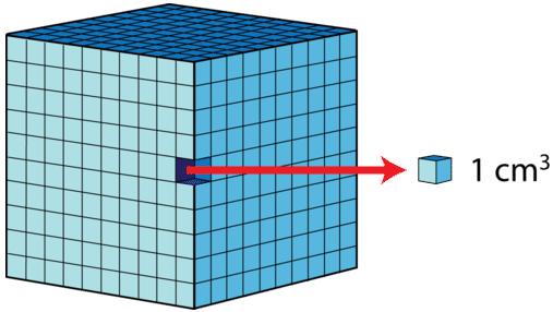
Because a cube has 3 sides, each side is subject to the conversion of \(1 \: \text{m}\) to \(100 \: \text{cm}\). Since 100 cubed is equal to 1 million \(\left( 10^6 \right)\), there are \(10^6 \: \text{cm}^3\) in \(1 \: \text{m}^3\). Two convenient volume units are the liter (which is equal to a cubic decimeter) and the milliliter, which is equal to a cubic centimeter. The conversion factor would be:
\[\left( \frac{1 \: \text{dm}}{10 \: \text{cm}} \right)^3 = \frac{1 \: \text{dm}^3}{1000 \: \text{cm}^3} = 1\nonumber \]
There are thus \(1000 \: \text{cm}^3\) in \(1 \: \text{dm}^3\), which is the same thing as saying there are \(1000 \: \text{mL}\) in \(1 \: \text{L}\).

Example \(\PageIndex{1}\)
Convert \(3.6 \times 10^8 \: \text{mm}^3\) to \(\text{mL}\).
Solution
Step 1: List the known quantities and plan the problem.
Known
- \(1 \: \text{m} = 1000 \: \text{mm}\)
- \(1 \: \text{mL} = 1 \: \text{cm}^3\)
- \(1 \: \text{m} = 100 \: \text{cm}\)
Unknown
This problem requires multiple steps and the technique for converting with derived units. Simply proceed one step at a time: \(\text{mm}^3\) to \(\text{m}^3\) to \(\text{cm}^3 = \text{mL}\).
Step 2: Calculate.
\[3.6 \: \text{mm}^3 \times \left( \frac{1 \: \text{m}}{1000 \: \text{mm}} \right)^3 \times \left( \frac{100 \: \text{cm}}{1 \: \text{m}} \right)^3 \times \frac{1 \: \text{mL}}{1 \: \text{cm}^3} = 0.0036 \: \text{mL} \nonumber\nonumber \]
Numerically, the steps are to divide 3.6 by \(10^9\), followed by multiplying by \(10^6\). You may find that you can shorten the problem by a step by first determining the conversion factor from \(\text{mm}\) to \(\text{cm}\), and using that instead of first converting to \(\text{m}\). There are \(10 \: \text{mm}\) in \(1 \: \text{cm}\).
\[3.6 \: \text{mm}^3 \times \left( \frac{1 \: \text{cm}}{10 \: \text{mm}} \right)^3 \times \frac{1 \: \text{mL}}{1 \: \text{cm}^3} = 0.0036 \: \text{mL} \nonumber\nonumber \]
In this case, 3.6/1000 gives the same result of 0.0036.
Step 3: Think about your result.
Cubic millimeters are much smaller than cubic centimeters, so the final answer is much less than the original number of \(\text{mm}^3\).
Summary
- A derived unit is a unit that results from a mathematical combination of SI base units.
- Calculations involving derived units follow the same principles as other unit conversion calculations.
Review
- What is a derived unit?
- Convert 0.00722 km3 to m3
- Convert 129 cm3 to L
- Convert 4.9 × 105 μm3 to mm3

