11.1: Absorption of Light

Introduction

The d-orbital splitting in coordination complexes results in a gap (\(\Delta\)) that happens to be just the right magnitude to absorb visible light. Because metal complexes can absorb visible light, they display an array of colors. Not only is the color attractive to the eye, it is an indication of the chemical and physical properties of the metal complex. The color (like the magnitude of \(\Delta\)) depends on the identity of the metal ion, the coordination geometry, and the ligand identity. Chemists don't just "look" at color, though - we measure it using electronic absorption spectroscopy. This is usually done in a lab using a UV-visible spectrophotometer.

An example of such a measurement is shown below in Figure \(\PageIndex{1}\) for a Cu(II) complex. The sample appears a pink color to the eye, and when it is measured using a UV-visible spectrometer, it is shown to absorb visible light at approximately 530 nm. The absorption spectrum can indicate the oxidation state of Cu, the ligands bound to the Cu(II) ion, and the coordination geometry. The color of the solution in Figure \(\PageIndex{1}\) is a shade of pink.

Figure \(\PageIndex{1}\): A UV-visible spectrum of a Cu(II)-peptide complex. A photo of the sample shows its pink color. The splitting diagram for its approximation as an octahdral complex is shown, where an electronic transition from \(t_{2g}\) to \(e_g\) is shown. (CC-BY-NC-SA; Kathryn Haas)

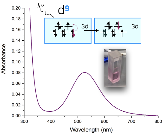
We observe the complementary color of light absorbed

The absorption spectrum shown above in Figure \(\PageIndex{1}\) is a simple case in which only one absorption band is observed in the visible region of the spectrum. In a simple case like this, the color of a complex can be predicted as the complementary color of the light absorbed by the solution. When a solution or object absorbs a certain wavelength, we see the complementary color; or the color opposite to the absorbed wavelength on the color wheel in Figure \(\PageIndex{2}\). In the case of the Cu(II) complex spectrum shown in Figure \(\PageIndex{1}\), the color of the light absorbed at 530 nm is green, and the predicted color observed is pink.

Figure \(\PageIndex{2}\): Color wheel with approximate wavelengths of colors. (CC-BY-NC-SA; Kathryn Haas)

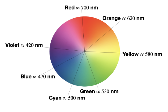
The table below lists the approximate colors of absorption corresponding to wavelengths of light absorbed, and gives similar information to that deduced from Figure \(\PageIndex{2}\).

Table \(\PageIndex{1}\): Approximate wavelengths of absorption and their complementary colors observed. * This prediction is limited to simple cases where there is only one absorption band in the visible spectrum.

\(\lambda\) absorbed	E (cm\(^{-1}\))	E (eV)	Approximate color absorbed	Predicted color observed (by eye)
\(> 700\) nm	\(< 14,000 \frac{1}{\text{cm}}\)	\( < 1.77\) eV	Infrared	not observable
\(\approx 700-635\) nm	\(\approx 14,300- 16,000\frac{1}{\text{cm}}\)	\( \approx 1.77-1.95\) eV	Red	Green
\(\approx 635-590\) nm	\(\approx 15,700- 16,900 \frac{1}{\text{cm}}\)	\( \approx 1.95-2.10\) eV	Orange	Blue
\(\approx 590-560\) nm	\(\approx 16,900-17,900 \frac{1}{\text{cm}}\)	\( \approx 2.10-2.21\) eV	Yellow	Violet
\(\approx 560-520\) nm	\(\approx 17,900- 19,200 \frac{1}{\text{cm}}\)	\( \approx 2.21-2.38\) eV	Green	Red
\(\approx 520-490\) nm	\(\approx 19,200- 20,400 \frac{1}{\text{cm}}\)	\( \approx 2.38-2.53\) eV	Cyan	Red-Orange
\(\approx 490-450\) nm	\(\approx 20,400- 22,200 \frac{1}{\text{cm}}\)	\( \approx 2.53-2.76\) eV	Blue	Orange
\(400-450\) nm	\(\approx 22,200- 25,000 \frac{1}{\text{cm}}\)	\( \approx 2.76-3.10\) eV	Violet	Yellow
<400 nm	\(> 25,000 \frac{1}{\text{cm}}\)	\( > 3.10\) eV	Ultraviolet (UV)	not observable

Energy of electronic absorption

The absorption spectrum of a metal complex can be used to calculate the splitting energy, \(\Delta\), when the absorption corresponds to a \(d \rightarrow d \) transition. Let's use the \(d^9\) Cu(II) complex (discussed above) as an example. A \(d^9\) metal ion has only one visible-light \(d \rightarrow d\) transition. Let's assume that the coordination geometry is approximately octahedral (although it is actually a Jahn-Teller distorted octahedron, and more like a square plane). If we assume it's octahedral, then the \(d\)-orbital splitting diagram (see Figure \(\PageIndex{1}\)) leads us to expect one electronic transition: an electron is excited from the \(t_{2g}\) to \(e_g\). The energy absorbed is equal to the energy of the \(\Delta\).

Many cases are not as simple as a \(d^9\) octahedral case because there are multiple possible electronic transitions, and also multiple absorption bands in the UV-vis spectrum. In these more complex cases, the actual energy of the transition are affected by differences in electron-electron repulsion energies in the ground state and the excited states. We will learn how to account for multiple possible excited states and electron-electron repulsions using Tanabe-Sugano diagrams later in this chapter.