2.2: The Reliability of a Measurement
- Page ID
- 25444
\( \newcommand{\vecs}[1]{\overset { \scriptstyle \rightharpoonup} {\mathbf{#1}} } \)
\( \newcommand{\vecd}[1]{\overset{-\!-\!\rightharpoonup}{\vphantom{a}\smash {#1}}} \)
\( \newcommand{\dsum}{\displaystyle\sum\limits} \)
\( \newcommand{\dint}{\displaystyle\int\limits} \)
\( \newcommand{\dlim}{\displaystyle\lim\limits} \)
\( \newcommand{\id}{\mathrm{id}}\) \( \newcommand{\Span}{\mathrm{span}}\)
( \newcommand{\kernel}{\mathrm{null}\,}\) \( \newcommand{\range}{\mathrm{range}\,}\)
\( \newcommand{\RealPart}{\mathrm{Re}}\) \( \newcommand{\ImaginaryPart}{\mathrm{Im}}\)
\( \newcommand{\Argument}{\mathrm{Arg}}\) \( \newcommand{\norm}[1]{\| #1 \|}\)
\( \newcommand{\inner}[2]{\langle #1, #2 \rangle}\)
\( \newcommand{\Span}{\mathrm{span}}\)
\( \newcommand{\id}{\mathrm{id}}\)
\( \newcommand{\Span}{\mathrm{span}}\)
\( \newcommand{\kernel}{\mathrm{null}\,}\)
\( \newcommand{\range}{\mathrm{range}\,}\)
\( \newcommand{\RealPart}{\mathrm{Re}}\)
\( \newcommand{\ImaginaryPart}{\mathrm{Im}}\)
\( \newcommand{\Argument}{\mathrm{Arg}}\)
\( \newcommand{\norm}[1]{\| #1 \|}\)
\( \newcommand{\inner}[2]{\langle #1, #2 \rangle}\)
\( \newcommand{\Span}{\mathrm{span}}\) \( \newcommand{\AA}{\unicode[.8,0]{x212B}}\)
\( \newcommand{\vectorA}[1]{\vec{#1}} % arrow\)
\( \newcommand{\vectorAt}[1]{\vec{\text{#1}}} % arrow\)
\( \newcommand{\vectorB}[1]{\overset { \scriptstyle \rightharpoonup} {\mathbf{#1}} } \)
\( \newcommand{\vectorC}[1]{\textbf{#1}} \)
\( \newcommand{\vectorD}[1]{\overrightarrow{#1}} \)
\( \newcommand{\vectorDt}[1]{\overrightarrow{\text{#1}}} \)
\( \newcommand{\vectE}[1]{\overset{-\!-\!\rightharpoonup}{\vphantom{a}\smash{\mathbf {#1}}}} \)
\( \newcommand{\vecs}[1]{\overset { \scriptstyle \rightharpoonup} {\mathbf{#1}} } \)
\( \newcommand{\vecd}[1]{\overset{-\!-\!\rightharpoonup}{\vphantom{a}\smash {#1}}} \)
\(\newcommand{\avec}{\mathbf a}\) \(\newcommand{\bvec}{\mathbf b}\) \(\newcommand{\cvec}{\mathbf c}\) \(\newcommand{\dvec}{\mathbf d}\) \(\newcommand{\dtil}{\widetilde{\mathbf d}}\) \(\newcommand{\evec}{\mathbf e}\) \(\newcommand{\fvec}{\mathbf f}\) \(\newcommand{\nvec}{\mathbf n}\) \(\newcommand{\pvec}{\mathbf p}\) \(\newcommand{\qvec}{\mathbf q}\) \(\newcommand{\svec}{\mathbf s}\) \(\newcommand{\tvec}{\mathbf t}\) \(\newcommand{\uvec}{\mathbf u}\) \(\newcommand{\vvec}{\mathbf v}\) \(\newcommand{\wvec}{\mathbf w}\) \(\newcommand{\xvec}{\mathbf x}\) \(\newcommand{\yvec}{\mathbf y}\) \(\newcommand{\zvec}{\mathbf z}\) \(\newcommand{\rvec}{\mathbf r}\) \(\newcommand{\mvec}{\mathbf m}\) \(\newcommand{\zerovec}{\mathbf 0}\) \(\newcommand{\onevec}{\mathbf 1}\) \(\newcommand{\real}{\mathbb R}\) \(\newcommand{\twovec}[2]{\left[\begin{array}{r}#1 \\ #2 \end{array}\right]}\) \(\newcommand{\ctwovec}[2]{\left[\begin{array}{c}#1 \\ #2 \end{array}\right]}\) \(\newcommand{\threevec}[3]{\left[\begin{array}{r}#1 \\ #2 \\ #3 \end{array}\right]}\) \(\newcommand{\cthreevec}[3]{\left[\begin{array}{c}#1 \\ #2 \\ #3 \end{array}\right]}\) \(\newcommand{\fourvec}[4]{\left[\begin{array}{r}#1 \\ #2 \\ #3 \\ #4 \end{array}\right]}\) \(\newcommand{\cfourvec}[4]{\left[\begin{array}{c}#1 \\ #2 \\ #3 \\ #4 \end{array}\right]}\) \(\newcommand{\fivevec}[5]{\left[\begin{array}{r}#1 \\ #2 \\ #3 \\ #4 \\ #5 \\ \end{array}\right]}\) \(\newcommand{\cfivevec}[5]{\left[\begin{array}{c}#1 \\ #2 \\ #3 \\ #4 \\ #5 \\ \end{array}\right]}\) \(\newcommand{\mattwo}[4]{\left[\begin{array}{rr}#1 \amp #2 \\ #3 \amp #4 \\ \end{array}\right]}\) \(\newcommand{\laspan}[1]{\text{Span}\{#1\}}\) \(\newcommand{\bcal}{\cal B}\) \(\newcommand{\ccal}{\cal C}\) \(\newcommand{\scal}{\cal S}\) \(\newcommand{\wcal}{\cal W}\) \(\newcommand{\ecal}{\cal E}\) \(\newcommand{\coords}[2]{\left\{#1\right\}_{#2}}\) \(\newcommand{\gray}[1]{\color{gray}{#1}}\) \(\newcommand{\lgray}[1]{\color{lightgray}{#1}}\) \(\newcommand{\rank}{\operatorname{rank}}\) \(\newcommand{\row}{\text{Row}}\) \(\newcommand{\col}{\text{Col}}\) \(\renewcommand{\row}{\text{Row}}\) \(\newcommand{\nul}{\text{Nul}}\) \(\newcommand{\var}{\text{Var}}\) \(\newcommand{\corr}{\text{corr}}\) \(\newcommand{\len}[1]{\left|#1\right|}\) \(\newcommand{\bbar}{\overline{\bvec}}\) \(\newcommand{\bhat}{\widehat{\bvec}}\) \(\newcommand{\bperp}{\bvec^\perp}\) \(\newcommand{\xhat}{\widehat{\xvec}}\) \(\newcommand{\vhat}{\widehat{\vvec}}\) \(\newcommand{\uhat}{\widehat{\uvec}}\) \(\newcommand{\what}{\widehat{\wvec}}\) \(\newcommand{\Sighat}{\widehat{\Sigma}}\) \(\newcommand{\lt}{<}\) \(\newcommand{\gt}{>}\) \(\newcommand{\amp}{&}\) \(\definecolor{fillinmathshade}{gray}{0.9}\)- Define accuracy and precision
- Distinguish exact and uncertain numbers
- Correctly represent uncertainty in quantities using significant figures
- Apply proper rounding rules to computed quantities
Counting is the only type of measurement that is free from uncertainty, provided the number of objects being counted does not change while the counting process is underway. The result of such a counting measurement is an example of an exact number. If we count eggs in a carton, we know exactly how many eggs the carton contains. The numbers of defined quantities are also exact. By definition, 1 foot is exactly 12 inches, 1 inch is exactly 2.54 centimeters, and 1 gram is exactly 0.001 kilogram. Quantities derived from measurements other than counting, however, are uncertain to varying extents due to practical limitations of the measurement process used.
Reporting Measurements to Reflect Certainty
Scientific measurements are of no value (or at least, they're not really scientific) unless they are given with some statement of the errors they contain. If a poll reports that one candidate leads another by 5%, that may be politically useful for the winning candidate to point out. But all respectable polls are scientific, and report errors. If the error in measurement is plus or minus 10%, which indicates anything from the candidate leading by 15% to trailing by 5%, the poll really does not reliably tell who is in the lead. If the poll had an error of 1%, the leading candidate could make a more scientific case that for being in the lead (by a 4% to 6% margin, or 5% +/-1%).
The numbers of measured quantities, unlike defined or directly counted quantities, are not exact. Scientific measurements are reported so that every digit is certain except the last, which is estimated. All digits of a measured quantity, including the certain one, are called significant figures.
To measure the volume of liquid in a graduated cylinder, you should make a reading at the bottom of the meniscus, the lowest point on the curved surface of the liquid.

Refer to the illustration in Figure \(\PageIndex{1}\). The bottom of the meniscus in this case clearly lies between the 21 and 22 markings, meaning the liquid volume is certainly greater than 21 mL but less than 22 mL. The meniscus appears to be a bit closer to the 22-mL mark than to the 21-mL mark, and so a reasonable estimate of the liquid’s volume would be 21.6 mL. In the number 21.6, then, the digits 2 and 1 are certain, but the 6 is an estimate. Some people might estimate the meniscus position to be equally distant from each of the markings and estimate the tenth-place digit as 5, while others may think it to be even closer to the 22-mL mark and estimate this digit to be 7. Note that it would be pointless to attempt to estimate a digit for the hundredths place, given that the tenths-place digit is uncertain. In general, numerical scales such as the one on this graduated cylinder will permit measurements to one-tenth of the smallest scale division. The scale in this case has 1-mL divisions, and so volumes may be measured to the nearest 0.1 mL.
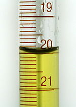
How much water (with yellow dye) does the graduated buret in Figure \(\PageIndex{2}\) contain?

Solution
The amount of water is somewhere between 19 ml and 20 ml according to the marked lines. By checking to see where the bottom of the meniscus lies, referencing the ten smaller lines, the amount of water lies between 19.8 ml and 20 ml. The next step is to estimate the uncertainty between 19.8 ml and 20 ml. Making an approximate guess, the level is less than 20 ml, but greater than 19.8 ml. We then report that the measured amount is approximately 19.9 ml. The graduated cylinder itself may be distorted such that the graduation marks contain inaccuracies providing readings slightly different from the actual volume of liquid present.
This concept holds true for all measurements, even if you do not actively make an estimate. If you place a quarter on a standard electronic balance, you may obtain a reading of 6.72 g. The digits 6 and 7 are certain, and the 2 indicates that the mass of the quarter is likely between 6.71 and 6.73 grams. The quarter weighs about 6.72 grams, with a nominal uncertainty in the measurement of ± 0.01 gram. If we weigh the quarter on a more sensitive balance, we may find that its mass is 6.723 g. This means its mass lies between 6.722 and 6.724 grams, an uncertainty of 0.001 gram. Every measurement has some uncertainty, which depends on the device used (and the user’s ability). All of the digits in a measurement, including the uncertain last digit, are called significant figures or significant digits. Note that zero may be a measured value; for example, if you stand on a scale that shows weight to the nearest pound and it shows “120,” then the 1 (hundreds), 2 (tens) and 0 (ones) are all significant (measured) values.
Accuracy and Precision
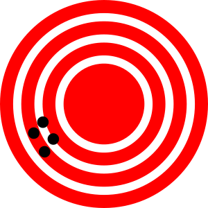
Scientists typically make repeated measurements of a quantity to ensure the quality of their findings and to know both the precision and the accuracy of their results. Measurements are said to be precise if they yield very similar results when repeated in the same manner. A measurement is considered accurate if it yields a result that is very close to the true or accepted value. Precise values agree with each other; accurate values agree with a true value. These characterizations can be extended to other contexts, such as the results of an archery competition (Figure \(\PageIndex{2}\)).
Figure \(\PageIndex{1}\) help to understand the difference between precision (small expected difference between multiple measurements) and accuracy (difference between the result and a known value).

Suppose a quality control chemist at a pharmaceutical company is tasked with checking the accuracy and precision of three different machines that are meant to dispense 10 ounces (296 mL) of cough syrup into storage bottles. She proceeds to use each machine to fill five bottles and then carefully determines the actual volume dispensed, obtaining the results tabulated in Table \(\PageIndex{2}\).
| Dispenser #1 | Dispenser #2 | Dispenser #3 |
|---|---|---|
| 283.3 | 298.3 | 296.1 |
| 284.1 | 294.2 | 295.9 |
| 283.9 | 296.0 | 296.1 |
| 284.0 | 297.8 | 296.0 |
| 284.1 | 293.9 | 296.1 |
Considering these results, she will report that dispenser #1 is precise (values all close to one another, within a few tenths of a milliliter) but not accurate (none of the values are close to the target value of 296 mL, each being more than 10 mL too low). Results for dispenser #2 represent improved accuracy (each volume is less than 3 mL away from 296 mL) but worse precision (volumes vary by more than 4 mL). Finally, she can report that dispenser #3 is working well, dispensing cough syrup both accurately (all volumes within 0.1 mL of the target volume) and precisely (volumes differing from each other by no more than 0.2 mL).
Summary
Quantities can be exact or measured. Measured quantities have an associated uncertainty that is represented by the number of significant figures in the measurement. The uncertainty of a calculated value depends on the uncertainties in the values used in the calculation and is reflected in how the value is rounded. Measured values can be accurate (close to the true value) and/or precise (showing little variation when measured repeatedly).
Glossary
- uncertainty
- estimate of amount by which measurement differs from true value
- significant figures
- (also, significant digits) all of the measured digits in a determination, including the uncertain last digit
- rounding
- procedure used to ensure that calculated results properly reflect the uncertainty in the measurements used in the calculation
- precision
- how closely a measurement matches the same measurement when repeated
- exact number
- number derived by counting or by definition
- accuracy
- how closely a measurement aligns with a correct value
Contributors and Attributions
Paul Flowers (University of North Carolina - Pembroke), Klaus Theopold (University of Delaware) and Richard Langley (Stephen F. Austin State University) with contributing authors. Textbook content produced by OpenStax College is licensed under a Creative Commons Attribution License 4.0 license. Download for free at http://cnx.org/contents/85abf193-2bd...a7ac8df6@9.110).

