8.1: Introduction

Contents 1 Introduction 2 Rutherford and The Nuclear Atom 3 The Quantization of Energy 3.1 The Ultraviolet Catastrophe 3.2 The Photoelectric Effect 3.3 The Spectrum of the Hydrogen Atom 4 Bohr's Theory of the Hydrogen Atom 4.1 Energy Levels of a General One-Electron Atom 4.2 The Need for a Better Theory 5 Particles of Light and Waves of Matter 6 The Uncertainty Principle 7 Wave Equations 8 The Hydrogen Atom 9 Many-Electron Atoms 10 Summary

“	The continuity if all dynamical effects was formerly taken for granted as the basis of all physical theories and, in close correspondence with Aristotle, was condensed in the well- known dogma-Natura non facit saltus- nature makes no leaps. However, present-day investigation has made a considerable breach even in this venerable stronghold if physical science. This time it is the principle if thermo- dynamics with which that theorem has been brought into collision by new facts, and unless all signs are misleading, the days if its validity are numbered. Nature does indeed seem to make jumps-and very extraordinary ones. Max Planck(1914)	”

IntroductionEdit

Physics seemed to be settling down quite satisfactorily in the late nineteenth century. A clerk in the U.S. Patent Office wrote a now-famous letter of resignation in which he expressed a desire to leave a dying agency, an agency that would have less and less to do in the future since most inventions had already been made. In 1894, at the dedication of a physics laboratory in Chicago, the famous physicist A. A. Michelson suggested that the more important physical laws all had been discovered, and "Our future discoveries must be looked for in the sixth decimal place." Thermodynamics, statistical mechanics, and electromagnetic theory had been brilliantly successful in explaining the behavior of matter. Atoms themselves had been found to be electrical, and undoubtedly would follow Maxwell's electromagnetic laws.

Then came x rays and radioactivity. In 1895, Wilhelm Rontgen (1845- 1923) evacuated a Crookes tube (Figure 1-11) so the cathode rays struck the anode without being blocked by gas molecules. Rontgen discovered that a new and penetrating form of radiation was emitted by the anode. This radiation, which he called x rays, traveled with ease through paper, wood, and flesh but was absorbed by heavier substances such as bone and metal. Rontgen demonstrated that x rays were not deflected by electric or magnetic fields and therefore were not beams of charged particles. Other scientists suggested that the rays might be electromagnetic radiation like light, but of a shorter wavelength. The German physicist Max von Laue proved this hypothesis 18 years later when he diffracted x rays with crystals.

In 1896, Henri Becquerel (1852–1908) observed that uranium salts emitted radiation that penetrated the black paper coverings of photographic plates and exposed the photographic emulsion. He named this behavior radioactivity. In the next few years, Pierre and Marie Curie isolated two entirely new, and radioactive, elements from uranium ore and named them polonium and radium. Radioactivity, even more than x rays, was a shock to physicists of the time. They gradually realized that radiation occurred during the breakdown of atoms, and that atoms were not indestructible but could decompose and decay into other kinds of atoms. The old certainties, and the hopes for impending certainties, began to fall away.

The radiation most commonly observed was of three kinds, designated alpha (α), beta (β), and gamma (γ). Gamma radiation proved to be electromagnetic radiation of even higher frequency (and shorter wavelength) than x rays. Beta rays, like cathode rays, were found to be beams of electrons. Electric and magnetic deflection experiments showed the mass of α radiation to be 4 amu and its charge to be +2; α particles were simply nuclei of helium, He.

The next certainty to slip away was the quite satisfying model of the atom that had been proposed by J. J. Thomson.

Rutherford and The Nuclear AtomEdit

File:Chemical Principles Fig 8.1.png

Figure 8-1

File:Chemical Principles Fig 8.2.png

Figure 8-2

File:Chemical Principles Fig 8.3.png

Figure 8-3

In Thomson's model of the atom all the mass and all the positive charge were distributed uniformly throughout the atom, with electrons embedded in the atom like raisins in a pudding. Mutual repulsion of electrons separated them uniformly. The resulting close association of positive and negative charges was reasonable. Ionization could be explained as a stripping away of some of the electrons from the pudding, thereby leaving a massive, solid atom with a positive charge.

In 1910, Ernest Rutherford (1871–1937) disproved the Thomson model, more or less by accident, while measuring the scattering of a beam of α particles by extremely thin sheets of gold and other heavy metals. (His experimental arrangement is shown in Figure 8-1.) He expected to find a relatively small deflection of particles, as would occur if the positive charge and mass of the atoms were distributed throughout a large volume in a uniform way (Figure 8-2a). What he observed was quite different, and wholly unexpected. In his own words:

"In the early days I had observed the scattering of α particles, and Dr. Geiger in my laboratory had examined it in detail. He found in thin pieces of heavy metal that the scattering was usually small, of the order of one degree. One day Geiger came to me and said, 'Don't you think that young Marsden, whom I am training in radioactive methods, ought to begin a small research?' Now I had thought that too, so I said, 'Why not let him see if any α particles can be scattered through a large angle?' I may tell you in confidence that I did not believe they would be, since we knew that the α particle was a very fast massive particle, with a great deal of energy, and you could show that if the scattering was due to the accumulated effect of a number of small scatterings, the chance of an α particle's being scattered backwards was very small. Then I remember two or three days later Geiger coming to me in great excitement and saying, 'We have been able to get some of the α particles coming backwards.' ... It was quite the most incredible event that has ever happened to me in my life. It was almost as incredible as if you fired a 15-inch shell at a piece of tissue paper and it came back and hit you."

Rutherford, Geiger, and Marsden calculated that this observed backscattering was precisely what would be expected if virtually all the mass and positive charge of the atom were concentrated in a dense nucleus at the center of the atom (Figure 8-2b). They also calculated the charge on the gold nucleus as 100 ± 20 (actually 79), and the radius of the gold nucleus as something less than 10⁻¹² cm (actually nearer to 10⁻¹³ cm).

The picture of the atom that emerged from these scattering experiments was of an extremely dense, positively charged nucleus surrounded by negative charges-electrons. These electrons inhabited a region with a radius 100,000 times that of the nucleus. The majority of the α particles passing through the metal foil were not deflected because they never encountered the nucleus. However, particles passing close to such a great concentration of charge would be deflected; and those few particles that happened to collide with the small target would be bounced back in the direction from which they had come.

The validity of Rutherford's model has been borne out by later investigations. An atom's nucleus is composed of protons and neutrons (Figure 8-3). Just enough electrons are around this nucleus to balance the nuclear charge. But this model of an atom cannot be explained by classical physics. What keeps the positive and negative charges apart? If the electrons were stationary, electrostatic attraction would pull them toward the nucleus to form a miniature version of Thomson's atom. Conversely, if the electrons were moving in orbits around the nucleus, things would be no better. An electron moving in a circle around a positive nucleus is an oscillating dipole when the atom is viewed in the plane of the orbit; the negative charge appears to oscillate up and down relative to the positive charge, By all the laws of classical electromagnetic theory, such an oscillator should broadcast energy as electromagnetic waves. But if this happened, the atom would lose energy, and the electron would spiral into the nucleus. By the laws of classical physics, the Rutherford model of the atom could not be valid. Where was the flaw?

The Quantization of EnergyEdit

Other flaws that were just as disturbing as Rutherford's impossibly stable atoms were appearing in physics at this time. By the turn of the century scientists realized that radio waves, infrared, visible light, and ultraviolet radiation (and x rays and y rays a few years later) were electromagnetic waves with different wavelengths. These waves all travel at the same speed, c, which is 2.9979 × l0⁸ m sec^-l or 186,000 miles sec^-l (This speed seems almost instantaneous until you recall that the slowness of light is responsible for the 1.3-sec delay each way in radio messages between the earth and the moon.) Waves such as these are described by their wavelength (designated by the Greek letter lambda, λ), amplitude, and frequency (designated by the Greek letter nu, ν), which is the number of cycles of a moving wave that passes a given point per unit of time (Figure 8-4). The speed of the wave, c, which is constant for all electromagnetic radiation, is the product of the frequency (the number of cycles per second or hertz, Hz) and the length of each cycle (the wavelength):

     c = νλ                                        (8-1)

The reciprocal of the wavelength is called the wave number, :

= 1/λ

Its units are commonly waves per centimeter, or cm⁻¹.

The electromagnetic spectrum as we know it is shown in Figure 8-5a. The scale is logarithmic rather than linear in wavelength; that is, it is in increasing powers of 10. On this logarithmic scale, the portion of the electromagnetic radiation that our eyes can see is only a small sector halfway between radio waves and gamma rays. The visible part of the spectrum is shown in Figure 8-5b.

Example 1

Light of wavelength 5000 Å (or 5 × 10^−5 cm) falls in the green region of the visible spectrum. Calculate the wave number, , corresponding to this wavelength.

Solution The wave number is equal to the reciprocal of the wavelength, so = 1/λ = 1/5 × 10^-5 cm = 0.2 × 10^5 cm^-1 = 2 × 10^4 cm^-1

The Ultraviolet CatastropheEdit

Classical physics gave physicists serious trouble even when they used it to try to explain why a red-hot iron bar is red. Solids emit radiation when they are heated. The ideal radiation from a perfect absorber and emitter of radiation is called blackbody radiation. The spectrum, or plot of relative intensity against frequency, of radiation from a red-hot solid is shown in Figure 8-6a. Since most of the radiation is in the red and infrared frequency regions, we see the color of the object as red. As the temperature is increased, the peak of the spectrum moves to higher frequencies, and we see the hot object as orange, then yellow, and finally white when enough energy is radiated through the entire visible spectrum.

The difficulty in this observation is that classical physics predicts that the curve will keep rising to the right rather than falling after a maximum. Thus there should be much more blue and ultraviolet radiation emitted than is actually observed, and all heated objects should appear blue to our eyes. This complete contradiction of theory by facts was called the ultraviolet catastrophe by physicists of the time.

In 1900, Max Planck provided an explanation for this paradox. To do this he had to discard a hallowed tenet of science-that variables in nature change in a continuous way (nature does not make jumps). According to classical physics, light of a certain frequency is emitted because charged objects- atoms or groups of atoms- in a solid vibrate or oscillate with that frequency. We could thus theoretically calculate the intensity curve of the spectrum if we knew the relative number of oscillators that vibrate with each frequency.All frequencies are thought to be possible, and the energy associated with a particular frequency depends only on how many oscillators are vibrating with that frequency . There should be no lack of high-frequency oscillators in the blue and ultraviolet regions.

Planck made the revolutionary suggestion that the energy of electromagnetic radiation comes in packages, or quanta. The energy of one package of radiation is proportional to the frequency of the radiation:

      E = hν                                             (8-2)

The proportionality constant, h, is known as Planck's constant and has the value 6.6262 × 10⁻³⁴ J sec. By Planck's theory, a group of atoms cannot emit a small amount of energy at a high frequency; high frequencies can be emitted only by oscillators with a large amount of energy, as given by E = hν. The probability of finding oscillators with high frequencies is therefore slight because the probability of finding groups of atoms with such unusually large vibrational energies is low. Instead of rising, the spectral curve falls at high frequencies, as in Figure 8-6.

Was Planck's theory correct, or was it only an ad hoc explanation to account for one isolated phenomenon? Science is plagued with theories that explain the phenomenon for which they were invented, and thereafter never explain another phenomenon correctly. Was the idea that electromagnetic energy comes in bundles of fixed energy that is proportional to frequency only another one-shot explanation?

The Photoelectric EffectEdit

Albert Einstein (1879–1955) provided another example of the quantization of energy, in 1905, when he successfully explained the photoelectric effect, in which light striking a metal surface can cause electrons to be given off. (Photocells in automatic doors use the photoelectric effect to generate the electrons that operate the door-opening circuits.) For a given metal there is a minimum frequency of light below which no electrons are emitted, no matter how intense the beam of light. To classical physicists it seemed nonsensical that for some metals the most intense beam of red light could not drive off electrons that could be ejected by a faint beam of blue light.

Einstein showed that Planck's hypothesis explained such phenomena beautifully. The energy of the quanta of light striking the metal, he said, is greater for blue light than for red. As an analogy, imagine that the low-frequency red light is a beam of Ping-Pong balls and that the high-frequency blue light is a beam of steel balls with the same velocity. Each impact of a quantum of energy of red light is too small to dislodge an electron; in our analogy, a steady stream of Ping-Pong balls cannot do what one rapidly moving steel ball can. These quanta of light were named photons. Because of the successful explanation of both the blackbody and photoelectric effects, physicists began recognizing that light behaves like particles as well as like waves.

Example 2

Consider once again the green light in Example 1. The relationship E = hν allows us to calculate the energy of one green photon. What is this energy in kilojoules? In kilojoules per mole of green photons?

Solution Let us assume that we know the wavelength to two significant digits, 5.0 X 10^−5 cm. The frequency, ν, of this green light is c = λν = 3.0 × 10^10 cm sec^-1 = (5.0 × 10^-5 cm) ν ν =   = 0.60 × 10^15 sec^-1     (or 0.60 × 10^15 Hz) The energy of one green photon, then, is E = hν   (6.63 × 10^-34 J sec)(0.60 × sec^-1)   4.0 × 10^-19 J, or 4.0 × 10^-22 kJ This is the energy of one green photon. To obtain the energy of a mole of green photons, we must multiply by Avogadro's number: E = (4.0 × 10^-22 kJ photon^-1)(6.02 × 10^-23 photons mole^-1)   = 2.4 × 10^2 kJ mole^-1

The Spectrum of the Hydrogen AtomEdit

The most striking example of the quantization of light, to a chemist, appears in the search for an explanation of atomic spectra. Isaac Newton (1642–1727) was one of the first scientists to demonstrate with a prism that white light is a spectrum of many colors, from red at one end to violet at the other. We know now that the electromagnetic spectrum continues on both sides of the small region to which our eyes are sensitive; it includes the infrared at low frequencies and the ultraviolet at high frequencies.

All atoms and molecules absorb light of certain characteristic frequencies. The pattern of absorption frequencies is called an absorption spectrum and is an identifying property of any particular atom or molecule. The absorption spectrum of hydrogen atoms is shown in Figure 8-7. The lowest-energy absorption corresponds to the line at 82,259 cm⁻¹. Notice that the absorption lines are crowded closer together as the limit of 109,678 cm⁻¹ is approached. Above this limit absorption is continuous.

If atoms and molecules are heated to high temperatures, they emit light of certain frequencies. For example, hydrogen atoms emit red light when they are heated. An atom that possesses excess energy (e.g., an atom that has been heated) emits light in a pattern known as its emission spectrum. A portion of the emission spectrum of atomic hydrogen is shown in Figure 8-8. Note that the lines occur at the same wave numbers in the two types of spectra.

If we look more closely at the emission spectrum in Figure 8-8, we see that there are three distinct groups of lines. These three groups or series are named after the scientists who discovered them. The series that starts at 82,259 cm⁻¹ and continues to 109,678 cm⁻¹ is called the Lyman series and is in the ultraviolet portion of the spectrum. The series that starts at 15,233 cm⁻¹ and continues to 27,420 cm⁻¹ is called the Balmer series and covers a large portion of the visible and a small part of the ultraviolet spectrum. The lines between 5332 cm⁻¹ and 12,186 cm⁻¹ are called the Paschen series and fall in the near-infrared region. The Balmer spectra of hydrogen from several stars are shown in Figure 8-9.

J. J. Balmer proved, in 1885, that the wave numbers of the lines in the Balmer spectrum of the hydrogen atom are given by the empirical relationship

       RH      n = 3, 4, 5, . . .                               (8-3)   

Later, Johannes Rydberg formulated a general expression that gives all of the line positions. This expression, called the Rydberg equation, is

       = RH                                  (8-4)

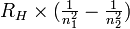
In the Rydberg equation n₁ and n₂ are integers, with n₂ greater than n₁; R_H is called the Rydberg constant and is known accurately from experiment to be 109,677.581 cm⁻¹.

Example 3

Calculate for the lines with n1 = 1 and n2 = 2, 3, and 4.

Solution n1 = 1, n2 = 2 line: n1 = 1, n2 = 3 line: n1 = 1, n2 = 4 line:

We see that the wave numbers obtained in Example 3 correspond to the first three lines in the Lyman series. Thus we expect that the Lyman series corresponds to lines calculated with n₁ = 1 and n₂ = 2, 3, 4, 5, . . . . We can check this by calculating the wave number for the line with n₂ = 1 and n₂ = ∞. n₁ = 1, n₂ = ∞ line:

The wave number 109,678 cm^-1 corresponds to the highest emission line in the Lyman series.

The wave number for n₁ = 2 and n₂ = 3 is

This corresponds to the first line in the Balmer series. Thus, the Balmer series corresponds to the n₁ = 2, n₂ = 3, 4, 5, 6, . . . lines. You probably would expect the lines in the Paschen series to correspond to n₁ = 3, n₂ = 4, 5, 6, 7, . . . They do. Now you should wonder where the lines are with n₁ = 4, n₂ = 5, 6, 7, 8, . . . , and n₁ = 5, n₂ = 6, 7, 8, 9, . . . . They are exactly where the Rydberg equation predicts they should be. The n = 4 series was discovered by Brackett and the n = 5 series was discovered by Pfund. The series with n = 6 and higher are located at very low frequencies and are not given special names.

The Rydberg formula, equation 8-4, is a summary of observed facts about hydrogen atomic spectra. It states that the wave number of a spectral line is the difference between two numbers, each inversely proportional to the square of an integer. If we draw a set of horizontal lines at a distance RH/n' down from a baseline, with n = 1, 2, 3, 4, . . ., then each spectral line in any of the hydrogen series is observed to correspond to the distance between two such horizontal lines in the diagram (Figure 8-10). The Lyman series occurs between line n = 1 and those above it; the Balmer series occurs between line n = 2 and those above it; the Paschen series occurs between line n = 3 and those above it; and the higher series are based on lines n = 4, 5, and so on. Is the agreement between this simple diagram and the observed wave numbers of spectral lines only a coincidence? Does the idea of a wave number of an emitted line being the difference between two "wave-number levels" have any physical significance, or is this just a convenient graphical representation of the Rydberg equation?

Bohr's Theory of the Hydrogen AtomEdit

In 1913, Niels Bohr (1885–1962) proposed a theory of the hydrogen atom that, in one blow, did away with the problem of Rutherford's unstable atom and gave a perfect explanation of the spectra we have just discussed.

There are two ways of proposing a new theory in science, and Bohr's work illustrates the less obvious one. One way is to amass such an amount of data that the new theory becomes obvious and self-evident to any observer. The theory then is almost a summary of the data. This is essentially the way Dalton reasoned from combining weights to atoms. The other way is to make a bold new assertion that initially does not seem to follow from the data, and then to demonstrate that the consequences of this assertion, when worked out, explain many observations. With this method, a theorist says, "You may not see why, yet, but please suspend judgment on my hypothesis until I show you what I can do with it." Bohr's theory is of this type.

Bohr answered the question of why the electron does not spiral into the nucleus by simply postulating that it does not. In effect, he said to classical physicists: "You have been misled by your physics to expect that the electron would radiate energy and spiral into the nucleus. Let us assume that it does not, and see if we can account for more observations than by assuming that it does." The observations that he explained so well are the wavelengths of lines in the atomic spectrum of hydrogen.

Bohr's model of the hydrogen atom is illustrated in Figure 8-11: an electron of mass m_e moving in a circular orbit at a distance r from a nucleus. If the electron has a velocity of v, it will have an angular momentum of m_evr. (To appreciate what angular momentum is, think of an ice skater spinning on one blade like a top. The skater begins spinning with his arms extended. As he brings his arms to his sides, he spins faster and faster. This is because, in the absence of any external forces, angular momentum is conserved. As the mass of the skater's arms comes closer to the axis of rotation, or as r decreases, the velocity of his arms must increase in order that the product mvr remain constant.) Bohr postulated, as the first basic assumption of his theory, that in a hydrogen atom there could only be orbits for which the angular momentum is an integral multiple of Planck's constant divided by 2:

m_evr

There is no obvious justification for such an assumption; it will be accepted only if it leads to the successful explanation of other phenomena. Bohr then showed that, with no more new assumptions, and with the laws of classical mechanics and electrostatics, his principle leads to the restriction of the energy of an electron in a hydrogen atom to the values

      E =    n = 1, 2, 3, 4, . . .                      (8-5)

The integer n is the same integer as in the angular momentum assumption, m_evr = n(h/ 2</math>\pi</math>); k is a constant that depends only on Planck's constant, h, the mass of an electron, m_e, and the charge on an electron, e:

k = 13.595 electron volts (eV)* atom^-1

= 1312 kJ mole^-1

The radius of the electron's orbit also is determined by the integer n:

      r = n2a0                               (8-6)

The constant, a₀, is called the first Bohr radius and is given in Bohr's theory by

a₀ = 0.529Å

The first Bohr radius is often used as a measure of length called the atomic unit, a.u.

The energy that an electron in a hydrogen atom can have is quantized, or limited to certain values, by equation 8-5. The integer, n, that determines these energy values is called the quantum number. When an electron is removed (ionized) from an atom, that electron is described as excited to the quantum state n = ∞. From equation 8-5, we see that as n approaches ∞, E approaches zero. Thus, the energy of a completely ionized electron has been chosen as the zero energy level. Because energy is required to remove an electron from an atom, an electron that is bound to an atom must have less energy that this, and hence a negative energy. The relative sizes of the first five hydrogen-atom orbits are compared in Figure 8-12.

Example 4

For a hydrogen atom, what is the energy, relative to the ionized atom, of the ground state, for which n = 1? How far is the electron from the nucleus in this state? What are the energy and radius of orbit of an electron in the first excited state, for which n = 2?

Solution The answers are E1 = = -1312 kJ mole^-1 E2 = = -328.0 kJ mole^-1 r1 = 1^2 × 0.529 Å = 0.529 Å r2 = 2^2 × 0.529 Å = 2.12 Å An electron volt is equal to the amount of energy an electron gains as it passes from a point of low potential to a point one volt higher in potential (1 eV = 1.6022 × 10^−19 J).

Example 5

Using the Bohr theory, calculate the ionization energy of the hydrogen atom.

Solution The ionization energy, IE, is that energy required to remove the electron, or to go from quantum state n = 1 to n = ∞. This energy is IE = E∞ - E1 = 0.00 - (- 1312 kJ mole^-1)   = + 1312 kJ

Example 6

Diagram the energies available to the hydrogen atom as a series of horizontal lines. Plot the energies in units of k for simplicity. Include at least the first eight quantum levels and the ionization limit. Compare your result with Figures 8-10 and 8-13. Try this one yourself.

In the second part of his theory, Bohr postulated that absorption and emission of energy occur when an electron moves from one quantum state to another. The energy emitted when an electron drops from state n₂ to a lower quantum state n₁ is the difference between the energies of the two states:

      ΔE = E1 - E2 = -k                               (8-7)

The light emitted is assumed to be quantized in exactly the way predicted from the blackbody and photoelectric experiments of Planck and Einstein:

      |ΔE| = hv = hc                       (8-8)

If we divide equation 8-7 by hc to convert from energy to wave number units, we obtain the Rydberg equation,

Recall that the experimental value of R_H is 109,677.581 cm^-1.

The graphic representation of the Rydberg equation, Figure 8-10, now is seen to be an energy-level diagram of the possible quantum states of the hydrogen atom. We can see why light is absorbed or emitted only at specific wave numbers. The absorption of light, or the heating of a gas, provides the energy for an electron to move to a higher orbit. Then the excited hydrogen atom can emit energy in the form of light quanta when the electron falls back to a lower-energy orbit. From this emission come the different series of spectral lines:

1. The Lyman series of lines arises from transitions from the n = 2, 3, 4, . . . levels to the ground state (n = 1)

2. The Balmer series arises from transitions from the n = 3, 4, 5, . . . levels to the n = 2 level.

3. The Paschen series arises from transitions from the n = 4, 5, 6, . . . levels to the n = 3 level.

An excited hydrogen atom in quantum state n = 8 may drop directly to the ground state and emit photon in the Lyman series, or it may drop first to n = 3, emit a photon in the Paschen series, and then drop to n = 1 and emit a photon in the Lyman series. The frequency of each photon depends on the energy difference between levels:

ΔE = E_a - E_b = hv

By cascading down the energy levels, the electron in one excited hydrogen atom can successively emit photons in several series. Therefore, all series are present in the emission spectrum from hot hydrogen. However, when measuring the absorption spectrum of hydrogen gas at lower temperatures we find virtually all the hydrogen atoms in the ground state. Therefore, almost all the absorption will involve transitions from n = 1 to higher states, and only the Lyman series will be observed.

Energy Levels of a General One-Electron AtomEdit

Bohr's theory can also be used to calculate the ionization energy and spectral lines of any atomic species possessing only one electron (e.g., He⁺, Li²⁺, Be³⁺ ). The energy of a Bohr orbit depends on the square of the charge on the atomic nucleus (Z is the atomic number):

E =

where

k = 13.595 eV or 1312 kJ mole^-1

n = 1, 2, 3, 4, . . . ∞

The equation reduces to equation 8-5 in the case of atomic hydrogen (Z = 1).

Example 7

Calculate the third ionization energy of a lithium atom.

Solution A lithium atom is composed of a nucleus of charge +3 (Z = 3) and three electrons. The first ionization energy, IE1, of an atom with more than one electron is the energy required to remove one electron. For lithium, Li(g) → Li^+(g) + e^-    ΔE = IE1 The energy needed to remove an electron from the unipositive ion, Li^+, is defined as the second ionization energy, IE2, of lithium, Li(g) → Li^2+(g) + e^-    ΔE = IE2 and the third ionization energy, IE3, of lithium is the energy required to remove the one remaining electron from Li^2+. For lithium, Z = 3 and IE3 = (3)^2(13.595 eV) = 122.36 eV. (The experimental value is 122.45 eV.)

The Need for a Better TheoryEdit

The Bohr theory of the hydrogen atom suffered from a fatal weakness: It explained nothing except the hydrogen atom and any other combination of a nucleus and one electron. For example, it could account for the spectra of He⁺ and Li²⁺, but it did not provide a general explanation for atomic spectra. Even the alkali metals (Li, Na, K, Rb, Cs), which have a single valence electron outside a closed shell of inner electrons, produce spectra that are at variance with the Bohr theory. The lines observed in the spectrum of Li could be accounted for only by assuming that each of the Bohr levels beyond the first was really a collection of levels of different energies, as in Figure 8-13: two levels for n = 2, three levels for n = 3, four for n = 4, and so on. The levels for a specific n were given letter symbols based on the appearance of the spectra involving these levels: s for "sharp," p for "principal," d for "diffuse," and f for "fundamental."

Arnold Sommerfeld (1868–1951) proposed an ingenious way of saving the Bohr theory. He suggested that orbits might be elliptical as well as circular. Furthermore, he explained the differences in stability of levels with the same principal quantum number, n, in terms of the ability of the highly elliptical orbits to bring the electron closer to the nucleus (Figure 8-14). For a point nucleus of charge +1 in Hydrogen, the energies of all levels with the same n would be identical. But for a nucleus of +3 screened by an inner shell of two electrons Li, an electron in an outer circular orbit would experience a net attraction of +1, whereas one in a highly elliptical orbit would penetrate the screening shell and feel a charge approaching +3 for part of its traverse. Thus, the highly elliptical orbits would have the most additional stability illustrated in Figure 8-13. The s orbits, being the most elliptical of all in Sommerfeld's model, would be much more stable than the others in the set of common n.

The Sommerfeld scheme led no further than the alkali metals. Again an impasse was reached, and an entirely fresh approach was needed.

Particles of Light and Waves of MatterEdit

At the beginning of the twentieth century, scientists generally believed that all physical phenomena could be divided into two distinct and exclusive classes. The first class included all phenomena that could be described by laws of classical, or Newtonian, mechanics of motion of discrete particles.

The second class included all phenomena showing the continuous properties of waves.

One outstanding property of matter, apparent since the time of Dalton, is that it is built of discrete particles. Most material substances appear to be continuous: water, mercury, salt crystals, gases. But if our eyes could see the nuclei and electrons that constitute atoms, and the fundamental particles that make up nuclei, we would discover quickly that every material substance in the universe composed of a certain number of these basic units and therefore is quantized. Objects appear continuous only because of the minuteness of the individual units.

In contrast, light was considered to be a collection of waves traveling through space at a constant speed; any combination of energies and frequencies was possible. However, Planck, Einstein, and Bohr showed that light when observed under the right conditions, also behaves as though it occurs in particles, or quanta.

In 1924, the French physicist Louis de Broglie (b. 1892) advanced the complementary hypothesis that all matter possesses wave properties. De Broglie pondered the Bohr atom, and asked himself where, in nature, quantization of energy occurs most naturally. An obvious answer is in the vibration of a string with fixed ends. A violin string can vibrate with only a selected set of frequencies: a fundamental tone with the entire string vibrating as a unit, and overtones of shorter wavelengths. A wavelength in which the vibration fails to come to a node (a place of zero amplitude) at both ends of the string would be an impossible mode of vibration (Figure 8-15). The vibration of a string with fixed ends is quantized by the boundary conditions that the ends cannot move.

Can the idea of standing waves be carried over to the theory of the Bohr atom? Standing waves in a circular orbit can exist only if the circumference of the orbit is an integral number of wavelengths (Figure 8-15c, d). If it is not, waves from successive turns around the orbit will be out of phase and will cancel. The value of the wave amplitude at 10° around the orbit from a chosen point will not be the same as at 370° or 730°, yet all these represent the same point in the orbit. Such ill-behaved waves are not single-valued at any point on the orbit: Single-valuedness is a boundary condition on acceptable waves.

For single-valued standing waves around the orbit, the circumference is an integer, n, times the wavelength:

2r = nλ

But from Bohr's original assumption about angular momentum,

2r = n

Therefore, the idea of standing waves leads to the following relationship between the mass of the electron m_e its velocity, v, and its wavelength, λ:

      λ =                              (8-10)

De Broglie proposed this relationship as a general one. With every particle, he said, there is associated a wave. The wavelength depends on the mass of the particle and how fast it is moving. If this is so, the same sort of diffraction from crystals that von Laue observed with x rays should be produced with electrons.

In 1927, C. Davisson and L. H. Germer demonstrated that metal foils diffract a beam of electrons exactly as they diffract an x-ray beam, and that the wavelength of a beam of electrons is given correctly by de Broglie's relationship (Figure 8-16). Electron diffraction is now a standard technique for determining molecular structure.

Example 8

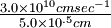
A typical electron diffraction experiment is conducted with electrons accelerated through a potential drop of 40,000 volts, or with 40,000 eV of energy. What is the wavelength of the electrons?

Solution First convert the energy, E, from electron volts to joules: E = 40,000 eV = 6.409 × 10^-15 J

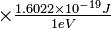
(This and several other useful conversion factors, plus a table of the values of frequently used physical constants, are in Appendix 2.) Since the energy is E = m_ev², the velocity of the electrons is

v =

  (1.407 × 10¹⁶ m² sec^-2)^1/2 = 1.186 × 10⁸ m sec^-1

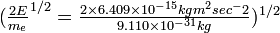
(In the expression E = m_ev², if the mass is in kilograms and the velocity is in m sec⁻¹, then the energy is in joules: 1 J equals 1 kg m² sec⁻² of energy. We used this conversion of units in the preceding step. The mass of the electron, m_e = 9.110 × 10⁻³¹ kg, is found in Appendix 2.) The momentum of the electron, m_ev, is

m_ev = 9.110 × 10^-31 kg × 1.186 × 10⁸ m sec^-1

  = 10.80 × 10^-23 kg m sec^-1

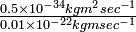
Finally, the wavelength of the electron is obtained from the de Broglie relationship:

λ =

  = 0.06130 × 10^-10 0.06130 × 10^-10 m

  = 0.06130 Å

So 40-kilovolt (kV) electrons produce the diffraction effects expected from waves with a wavelength of six-hundredths of an angstrom.

Such calculations are all very well, but the question remains: Are electrons waves or are they particles? Are light rays waves or particles? Scientists worried about these questions for years, until they gradually realized that they were arguing about language and not about science. Most things in our everyday experience behave either as what we would call waves or as what we would call particles, and we have created idealized categories and used the words wave and particle to identify them. The behavior of matter as small as electrons cannot be described accurately by these large-scale categories. Electrons, protons, neutrons, and photons are not waves, and they are not particles. Sometimes they act as if they were what we commonly call waves, and in other circumstances they act as if they were what we call particles. But to demand, "Is an electron a wave or a particle?" is pointless.

This wave-particle duality is present in all objects; it is only because of the scale of certain objects that one behavior predominates and the other is negligible. For example, a thrown baseball has wave properties, but a wavelength so short we cannot detect it.

Example 9

A 200-g baseball is thrown with a speed of 30 m sec^−1 Calculate its de Broglie wavelength.

Solution The answer is λ = 1.1 × 10^−34 m = 1.1 × 10^−24 Å.

Example 10

How fast (or rather, how slowly) must a 200-g baseball travel to have the same de Broglie wavelength as a 40-kV electron?

Solution The wavelength of a 40-kV electron is 0.0613 Å. v = =   = 0.540 × 10^-21 m sec^-1 = 1.70 × 10^-4 Å year^-1 Such a baseball would take over 10,000 years to travel the length of a carbon-carbon bond, 1.54 Å. This sort of motion is completely outside our experience with baseballs; thus we never regard baseballs as having wave properties.

The Uncertainty PrincipleEdit

One of the most important consequences of the dual nature of matter is the uncertainty principle, proposed in 1927 by Werner Heisenberg (1901–1976). This principle states that you cannot know simultaneously both the position and the momentum of any particle with absolute accuracy. The product of the uncertainty in position, , and in momentum, , will be equal to or greater than Planck's constant divided by 4:

      [Δx][Δ(mvx)] ≥                                 (8-11)

We can understand this principle by considering how we determine the position of a particle. If the particle is large, we can touch it without disturbing it seriously. If the particle is small, a more delicate means of locating it is to shine a beam of light on it and observe the scattered rays. Yet light acts as if it were made of particles - photons - with energy proportional to frequency: E = hν. When we illuminate the object, we are pouring energy on it. If the object is large, it will become warmer; if the object is small enough, it will be pushed away and its momentum will become uncertain. The least interference that we can cause is to bounce a single photon off the object and watch where the photon goes. Now we are caught in a dilemma. The detail in an image of an object depends on the fineness of the wavelength of the light used to observe the object. (The shorter the wavelength, the more detailed the image.) But if we want to avoid altering the momentum of the atom, we have to use a low-energy photon. However, the wavelength of the low-energy photon would be so long that the position of the atom would be unclear. Conversely, if we try to locate the atom accurately by using a short-wavelength photon, the energy of the photon sends the atom ricocheting away with an uncertain momentum (Figure 8-17). We can design an experiment to obtain an accurate value of either an atom's momentum or its position, but the product of the errors in these quantities is limited by equation 8-11.

Example 11

Suppose that we want to locate an electron whose velocity is 1.00 × 10^6 m sec^−1 by using a beam of green light whose frequency is 0.600 × 10^15 sec^−1. How does the energy of one photon of such light compare with the energy of the electron to be located?

Solution The energy of the electron is E =   = 4.56 × 10^-19 J But the energy of the photon is almost as large: Ep = hν = 6.6262 × 10^-34 J sec × 0.600 × 10^15 sec^-1   = 3.97 × 10^-19 J

Finding the position and momentum of such an electron with green light is as questionable a procedure as finding the position and momentum of one billiard ball by striking it with another. In either case, you detect the particle at the price of disturbing its momentum. As a final difficulty, green light is a hopelessly coarse yardstick for finding objects of atomic dimensions. An atom is about 1 Å in radius, whereas the wavelength of green light is around 5000 Å. Shorter wavelengths make the energy quandary worse.

We do not see the uncertainty limitations in large objects because of the sizes of the masses and velocities involved. Compare the following two problems.

Example 12

An electron is moving with ~ velocity of 10^6 m sec^−1 Assume that we can measure its position to 0.01 Å, or 1% of a typical atomic radius. Compare the uncertainty in its momentum, p, with the momentum of the electron itself.

Solution The uncertainty in position is Δx ≅ 0.01 Å = 0.01 × 10^−10m. The momentum of the electron is approximately p = mev ≅ 10^-30 kg × 10^6 m sec^-1 = 10^-24 kg m sec^-1 By the Heisenberg uncertainty principle, the uncertainty in the knowledge of the momentum is Δp = ≅ ≅ 0.5 × 10^-22 kg m sec^-1 The uncertainty in the momentum of the electron is 50 times as great as the momentum itself!

Example 13

A baseball of mass 200 g is moving with a velocity of 30 m sec^−1. If we can locate the baseball with an error equal in magnitude to the wavelength of light used (e.g., 5000 Å), how will the uncertainty in momentum compare with the total momentum of the baseball?

Solution The momentum, p, of the baseball is 6 kg m sec^−1, and Δp = 1 × 10^−28 kg m sec^−1. The intrinsic uncertainty in the momentum is only one part in 10^28, far below any possibility of detection in an experiment.

Wave EquationsEdit

In 1926, Erwin Schrödinger (1887–1961) proposed a general wave equation for a particle. The mathematics of the Schrödinger equation is beyond us, but the mode of attack, or the strategy of finding its solution, is not. If you can see how physicists go about solving the Schrödinger equation, even though you cannot solve it yourself, then quantization and quantum numbers may be a little less mysterious. This section is an attempt to explain the method of solving a differential equation of motion* of the type that we encounter in quantum mechanics. We shall explain the strategy with the simpler analogy of the equation of a vibrating string.

The de Broglie wave relationship and the Heisenberg uncertainty principle should prepare you for the two main features of quantum mechanics that contrast it with classical mechanics:

1. Information about a particle is obtained by solving an equation for a wave.

2. The information obtained about the particle is not its position;

rather, it is the probability of finding the particle in a given region of space.

We can't say whether an electron is in a certain place around an atom, but we can measure the probability that it is there rather than somewhere else.

Wave equations are familiar in mechanics. For instance, the problem of the vibration of a violin string is solved in three steps:

1. Set up the equation of motion of a vibrating string. This equation will involve the displacement or amplitude of vibration, A (x), as a function of position along the string, x.

2. Solve the differential equation to obtain a general expression for amplitude. For a vibrating string with fixed ends, this general expression is a sine wave. As yet, there are no restrictions on wavelength or frequency of vibration.

3. Eliminate all solutions to the equation except those that leave the ends of the string stationary. This restriction on acceptable solutions of the wave equation is a boundary condition. Figure 8-15a shows solutions that fit this boundary condition of fixed ends of the string; Figure 8-15b shows solutions that fail. The only acceptable vibrations are those with λ = 2a/n, or = n/2a, in which n = 1, 2, 3, 4, .... The boundary conditions and not the wave equation are responsible for the quantization of the wavelengths of string vibration.

*Equations of motion are always differential equations because they relate the change in one quantity to the change in another, such as change in position to change in time.

Exactly the same procedure is followed in quantum mechanics:

1. Set up a general wave equation for a particle. The Schrödinger equation is written in terms of the function ψ_(x,v,z) (where ψ is the Greek letter psi), which is analogous to the amplitude, A_(x), in our violin-string analogy. The square of this amplitude, |ψ|², is the relative probability density of the particle at position (x, y, z). That is, if a small element of volume, dv, is located at (x, y, z), the probability of finding an electron within that element of volume is If |ψ|² dv.

2. Solve the Schrödinger equation to obtain the most general expression for ψ_{(x, y, z)}.

3. Apply the boundary conditions of the particular physical situation. If the particle is an electron in an atom, the boundary conditions are that |ψ|² must be continuous, single-valued, and finite everywhere. All these conditions are only common sense. First, probability functions do not fluctuate radically from one place to another; the probability of finding an electron a few thousandths of an angstrom from a given position will not be radically different from the probability at the original position. Second, the probability of finding an electron in a given place cannot have two different values simultaneously. Third, since the probability of finding an electron somewhere must be 100%, or 1.000, if the electron really exists, the probability at anyone point cannot be infinite.

We now shall compare the wave equation for a vibrating string and the Schrödinger wave equation for a particle. In this text you will not be expected to do anything with either equation, but you should note the similarities between them.

♦ Vibrating string. The amplitude of vibration at a distance x along the string is A_(x). The differential equation of motion is

                                 (8-12)

The general solution to this equation is a sine function

and the only acceptable solutions (Figure 8-15a) are those for which ,math>\textstyle\overline{\nu}</math> = n/2a, where n = 1, 2, 3, 4, ... , and for which the phase shift, α, is zero:

♦ Schrödinger equation. The square of the amplitude If(x.v.z>i' is the probability density of the particle at (x,), z). The differential equation is |ψ_{(x, y, z)}|² is the probability density of the particle at (x, y,z). The differential equation is

                                   (8-13)

V is the potential energy function at (x, y, z), and m_e is the mass of the electron.

Although solving equation 8-13 is not a simple process, it is purely a mathematical operation; there is nothing in the least mysterious about it. The energy, E, is the variable that is restricted or quantized by the boundary conditions on |ψ|². Our next task is to determine what the possible energy states are.

The Hydrogen AtomEdit

The sine function that is the solution of te equation for the vibrating string is characterized by one integral quantum muber: n = 1, 2, 3, 4, . . . . The first few acceptable sine functions are

These are the first four curves in Figure 8-15a.

An atom is three-dimensional, whereas the string has only length. The solutions of the Schrödinger equation for the hydrogen atom are characterized by three integer quantum numbers: n, l, and m. These arise when solving the equation for the wave function, Ψ, which is analogous to the function A_n(x) in the vibrating string analogy. In solving the Schrödinger equation, we divide it into three parts. The solution of the radial part describes how the wave function, Ψ, varies with distance from the center of the atom. If we borrow the customary coordinate system of the earth, an azimuthal part produces a function that reveals how Ψ varies with north or south latitude, or distance up or down from the equator of the atom. Finally, an angular part is a third function that suggests how the wave function varies with east-west longitude around the atom. The total wave function, Ψ, is the product of these three functions. The wave functions that are solutions to the Schrödinger equation for the hydrogen atom are called orbitals.

In the process of separating the parts of the wave function, a constant, n, appears in the radial expression, another constant, l, occurs in the radial and azimuthal expressions, and m appears in the azimuthal and angular expressions. The boundary conditions that give physically sensible solutions to these three equations are that each function (radial, azimuthal, and angular) be continuous, single-valued, and finite at all points. These conditions will not be met unless n, l, and m are integers, l is zero or a positive integer less than n, and m has a value from -l to + l. From a one-dimensional problem (the vibrating string) we obtained one quantum number. With a three-dimensional problem, we obtain three quantum numbers.

The principal quantum number, n, can be any positive integer: n = 1, 2, 3, 4, 5, . . . . The azimuthal quantum number, l, can have any integral value from 0 to n - 1. The magnetic quantum number, m, can have any integral value from -l to +l. The different quantum states that the electron can have are listed in Table 8-1. For one electron around an atomic nucleus, the energy depends only on n. Moreover, the energy expression is exactly the same as in the Bohr theory:

E_n =    ::k

For Z = 1 (the hydrogen atom), we have simply:

E_n =

where k = 13.595 eV or 1312 kJ mole⁻¹.

Quantum states, with l = 0, 1, 2, 3, 4, 5, . . ., are called the s, p, d, f, g, h, . . . states, in an extension of the old spectroscopic notation (Figure 8-13). The wave functions corresponding to s, p, d, . . . states are called s, p, d, . . . orbitals. All of the l states for the same n have the same energy in the hydrogen atom; the energy-level diagram is as in Figure 8-10.

Example 14

An electron in atomic hydrogen has a principal quantum number of 5. What are the possible values of l for this' electron? When l = 3, what are the possible values of m? What is the ionization energy (in electron volts) of this electron? What would it be in the same n state in He^+?

Solution With n = 5, l may have a value of 4, 3, 2, 1, or 0. For l = 3, there are seven possible values of m: 3, 2, 1, 0, -1, -2, -3. The ionization energy of the electron depends only on n, according to: IE = -En En = - IE = Since k = 13.6eV. the IE of an electron with n = 5 is IE = 0.544 eV In general, for one-electron atomic species: IE = -En En = IE = For HE^+, Z = 2: IE = For a He^+ electron with n = 5, we have IE = 4 × 0.544 eV = 2.18 eV

Each of the orbitals for the quantum states differentiated by n, l, and m in Table 8-1 corresponds to a different probability distribution function for the electron in space. The simplest such probability functions, for s orbitals (l = 0), are spherically symmetrical. The probability of finding the electron is the same in all directions but varies with distance from the nucleus. The dependence of Ψ and of the probability density |Ψ|² on the distance of the electron from the nucleus in the 1s orbital is plotted in Figure 8-18. You can see the spherical symmetry of this orbital more clearly in Figure 8-19. The quantity |Ψ|²dv can be thought of either as the probability of finding an electron in the volume element dv in one atom, or as the average electron density within the corresponding volume element in a great many different hydrogen atoms. The electron is no longer in orbit in the Bohr-Sommerfeld sense; rather, it is an electron probability cloud. Such probability density clouds are commonly used as pictorial representations of hydrogenlike atomic orbitals.

The 2s orbital is also spherically symmetrical, but its radial distribution function has a node, that is, zero probability, at r = 2 atomic units (I atomic unit is a₀ = 0.529 Å). The probability density has a crest at 4 atomic units, which is the radius of the Bohr orbit for n = 2. There is a high probability of finding an electron in the 2s orbital closer to or farther from the nucleus than r = 2, but there is no probability of ever finding it in the spherical shell at a distance r = 2 from the nucleus (Figure 8-20). The 3s orbital has two such spherical nodes, and the 4s has three. However, these details are not as important in explaining bonding as are the general observations that s orbitals are spherically symmetrical and that they increase in size as n increases.

There are three 2p orbitals: 2p_x, 2p_y, 2p_z. Each orbital is cylindrically symmetrical with respect to rotation around one of the three principal axes x, y, z, as identified by the subscript. Each 2p orbital has two lobes of high electron density separated by a nodal plane of zero density (Figures 8-21 and 8-22). The sign of the wave function, Ψ, is positive in one lobe and negative in the other. The 3p, 4p, and higher p orbitals have one, two, or more additional nodal shells around the nucleus (Figure 8-23); again, these details are of secondary importance. The significant facts are that the three p orbitals are mutually perpendicular, strongly directional, and increasing size as n increases.

The five d orbitals first appear for n = 3. For n = 3, l can be 0, 1, or 2, thus s, p, and d orbitals are possible. The 3d orbitals are shown in Figure 8-24. Three of them, d_xy, d_yz, and d_xz, are identical in shape but different in orientation. Each has four lobes of electron density bisecting the angles between principal axes. The remaining two are somewhat unusual: The d_x²-y² orbital has lobes of density along the x and y axes, and the d_z² orbital has lobes along the z axis, with a small doughnut or ring in the xy plane/ However, there is nothing sacrosanct about the z axis. The proper combination of wave functions of these five d orbitals will give us another set of five d orbitals in which the d_z² -like orbital points along the x axis, or the y axis. We could even combine the wave functions to produce a set of orbitals, all of which were alike but differently oriented. However, the set of orbitals, all of which were alike but differently oriented. However, the set that we have described, d_xy, d_yz, d_xz, d_x²-y² and d_z², is convenient and is used conventionally in chemistry. The sign of the wave function, Ψ, changes from lobe to lobe, as indicated in Figure 8-24.

The azimuthal quantum number l is related to the shape of the orbital, and is referred to as the orbital-shape quantum number: s orbitals with l = 0 are spherically symmetrical, p orbitals with l = 1 have plus and minus extensions along one axis, and d orbitals with l = 2 have extensions along two mutually perpendicular directions (Figure 8-25). The third quantum number, m, describes the orientation of the orbital in space. It is sometimes called the magnetic quantum number because the usual way of distinguishing between orbitals with different spatial orientations is to place the atoms in a magnetic field and to note the differences in energy produced in the orbitals. We will use the more descriptive term, orbital-orientation quantum number.

There is a fourth quantum number that has not been mentioned. Atomic spectra, and more direct experiments as well, indicate that an electron behaves as if it were spinning around an axis. Each electron has a choice of two spin states with spin quantum numbers, s = + or - . A complete description of the state of an electron in a hydrogen atom requires the specification of all four quantum numbers: n, l, m, and s.

Many-Electron AtomsEdit

It is possible to set up the Schrödinger wave equation for lithium, which has a nucleus and three electrons, or uranium, which has a nucleus and 92 electrons. Unfortunately, we cannot solve the differential equations. There is little comfort in knowing that the structure of the uranium atom is calculable in principle, and that the fault lies with mathematics and not with physics. Physicists and physical chemists have developed many approximate methods that involve guesses and successive approximations o solutions of the Schrödinger equation. Electronic computers have been of immense value in such successive approximations. But the advantage of Schrödinger's theory of the hydrogen atom is that it gives us a clear qualitative picture of the electronic structure of many-electron atoms without such additional calculations. Bohr's theory was too simple and could not do this, even with Sommerfeld's help.

The extension of the hydrogen-atom picture to many-electron atoms is one of the most important steps in understanding chemistry, and we shall reserve it for the next chapter. We shall begin by assuming that electronic orbitals for other atoms are similar to the orbitals for hydrogen and that they can be described by the same four quantum numbers and have analogous probability distributions. If the energy levels deviate from the ones for hydrogen (which they do), then we shall have to provide a persuasive argument, in terms of the hydrogenlike orbitals, for these changes.

SummaryEdit

Rutherford's scattering experiments showed the atom to be composed of an extremely dense, positively charged nucleus surrounded by electrons. The nucleus is composed of protons and neutrons. A proton has one positive charge and a mass of 1.67 × 10⁻²⁷ kg. A neutron is uncharged and has a mass of 1.67 × 10⁻²⁷ kg.

Radio waves, infrared, visible, and ultraviolet light, x rays and γ rays are electromagnetic waves with different wavelengths. The speed of light, c, equal to 2.9979 × 10¹⁰ cm sec⁻¹, is related to its wavelength (λ) and frequency (ν) by c = νλ. The wave number, , is the reciprocal of the wavelength, = 1/λ. Hot objects radiate energy (blackbody radiation). Planck proposed that the energy of electromagnetic radiation is quantized. The energy of a quantum of electromagnetic radiation is proportional to its frequency, E = hν, in which h is Planck's constant, 6.6262 × 10⁻³⁴ J sec. Electron ejection caused by light striking a metal surface is called the photoelectric effect. Photon is the name given to a quantum of light. The energy of a photon is equal to hν, in which ν is the frequency of the electromagnetic wave. The pattern of light absorption by an atom or molecule as a function of wavelength frequency or wave number is called absorption spectrum. The related pattern of light emission from an atom or molecule is called emission spectrum. The emission spectrum of atomic hydrogen is composed of several series of lines. The positions of these lines are given accurately by a single equation, the Rydberg equation,

=

in which is the wave number of a given line, R_H is the Rydberg constant, 109,677.581 cm⁻¹, and n₁ and n₂ are integers (n₂ is greater than n₁). The Lyman series is that group of lines with n₁ = 1 and n₂ = 2, 3, 4, . . . . The Balmer series has n₁ = 2 and n₂ = 3, 4, 5, . . ., and the Paschen series has n₁ = 3 and n₂ = 4, 5, 6, . . . .

Bohr pictured the hydrogen atom as containing an electron moving in a circular orbit around a central proton. He proposed that only certain orbits were allowed, corresponding to the following energies:

in which E is the energy of an electron in the atom (relative to an ionized state, H⁺ + e^-), k is a constant, equal to 13.595 eV atom⁻¹ or 1312 kJ mole⁻¹, and n is a quantum number that can take only integer values from 1 to ∞. The radius of a Bohr orbit is r = n²a₀, where a₀ is called the first Bohr radius; a₀ = 0.529 Å. One atomic unit of length equals a₀. The ground state of atomic hydrogen is the lowest energy state, where n = 1. Excited states correspond to n = 2, 3, 4, . . . . The energy levels in a general one-electron atomic species, such as He⁺ and Li²⁺, with atomic number Z, are given by

The wave nature of electrons was established when Davisson and Germer showed that metal foils diffract electrons in the same way that they diffract a beam of x rays. The wave-particle duality exhibited by electrons is present in all objects. For large objects (such as baseballs), particle behavior predominates to such an extent that wave properties are unimportant.

Heisenberg proposed that we cannot know both the position and the momentum of a particle with absolute accuracy. The product of the uncertainty in position, Δx, and momentum, Δ(mv), must be at least as large as h/4:

[Δx][Δ(mv_x)] ≥

The wave equation for a particle is called the Schrödinger equation. The solutions to the Schrödinger equation, |Ψ_(x,y,z)|², is the relative probability density of the particle at position _(x,y,z). A place where the amplitude of a wave is zero is called a node.

Solution of the Schrödinger equation for the hydrogen atom yields wave functions Ψ_(x,y,z) and discrete energy levels for the electron. The wave functions Ψ_(x,y,z) are called orbitals. An orbital is commonly represented as a probability density cloud, that is, a three-dimensional picture of |Ψ_(x,y,z)|². Three quantum numbers are obtained from solving the Schrödinger equation: the principal quantum number, n, can be any positive integer (n = 1, 2, 3, 4, . . . ); the azimuthal (or orbital-shape) quantum number, l, can have any integral value from 0 to n - 1; the magnetic (or orbital-orientation) quantum number, m, takes integral values from -l to + l. The energy levels depend only on n,

Wave functions with l = 0 are called s orbitals; those with l = 1 are called p orbitals; those with l = 2 are called d orbitals; those with l = 3, 4, 5, . . ., are called f, g, h, . . ., orbitals. A fourth quantum number is needed to interpret atomic spectra. It is the spin quantum number,s, which can be or