18.6: Bimolecular Processes

A second type of microscopic process which can result in a chemical reaction involves collision of two particles. Such a process is called a bimolecular process. A typical example of a bimolecular process is the reaction between nitrogen dioxide and carbon monoxide:

\[\text{ NO}_{\text{2}} + \text{CO}\rightarrow \text{NO} + \text{ CO}_{\text{2}} \nonumber \]

 

Here an O atom is transferred from NO₂ to CO when the two molecules collide.

Several factors affect the rate of a bimolecular reaction. The first of these is the frequency of collisions between the two reactant molecules. Suppose we have a single molecule of type A (shown in black in Figure \(\PageIndex{1}\)a, or in blue in the animation) moving around in a gas which otherwise consists entirely of molecules of kind B (indicated in white in the figure, light blue in the animation). If we double the concentration of B molecules (Figure 1b), the number of collisions during the same time period doubles, because there are now twice as many B molecules to get in the way. Similarly, if we put twice as many A molecules into the original container, each of them collides with B molecules the same number of times, again giving twice as many A-B collisions.

The argument in the previous paragraph applies to any bimolecular process. The reaction rate must always be directly proportional to the concentration of each of the two reacting species. Thus for the general bimolecular process, A + B → products, the rate equation must be first order in A and first order in B:

\[\text{Rate} = k (c_{A})(c_{B}) \nonumber \]

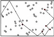
(a)A single black molecule moving among 50 white molecules collides with 5 of them in 1 s.

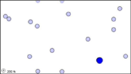
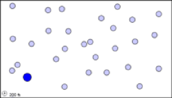
A single larger particle collides 6 times with a set of 14 smaller particles over a simulated time frame of 17200 fs.

(b) If the number of white molecules is doubled, the frequency collisions rises to 10 s^–1.

A single larger particle collides 14 times with a set of 28 smaller particles over a simulated time frame of 17200 fs.

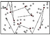
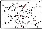
(c) Two black molecules moving among 50 white ones produce 10 collisions per second. The number of collisions can thus be seen to be proportional to both the concentration of white molecules and the concentration of black molecules.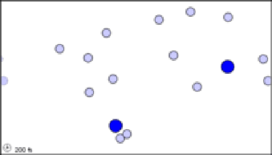

Two larger particles collide 15 times with a set of 14 smaller particles over a simulated time frame of 17200 fs.

Figure \(\PageIndex{1}\) The effect of concentration on the frequency of collisions. These still images show the number of collisions between a black particle and a collection of white particles. White particles that have been hit are displayed in color. The animations display the number of collisions that occur between the dark blue particles and a set of lighter blue particles over a simulated time frame of 17200 fs, though the animation is around 8 seconds long. When hit, a lighter blue particle changes to black, then red, then white, then purple at each subsequent hit, so to quantify total collisions more easily.

The animations above serve as another way of modeling what is occurring in the still images. Notice that, as in the still image, roughly twice as many collisions occur when there are two larger blue particles or twice as many small light blue particles, than in the first initial condition. Exact count shows this is not perfectly true though, as animation (a) has 6 collisions, while animation (b) and (c) have 14 and 15 respectively. This yields a factor of 2.3 and 2.5 respectively. This highlights an important point. When we say that doubling the amount of either substance should double the collisions, we mean collisions will, on average be doubled. Notice that the exact ratio between the animations at a specific time point fluctuates. Also, it is important to note that there are never more than 30 particles of either type in any of the simulations. When dealing with the scale of moles in an actual reaction, such a difference as 2 or 3 more collisions than predicted is vanishingly small.

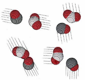
Collision of two molecules is a necessary but not a sufficient condition for a bimolecular process to occur. Returning to the reaction of NO₂ with CO, in which an O atom is transferred from the N atom to the C atom, we can see that the orientation of the two molecules as they collide is important. This introduces what is called a steric factor. None of the collisions depicted in Figure \(\PageIndex{2}\) would result in reaction, for example, because none of them involve close contact between the C atom in CO and one of the O’s in NO₂. For the reaction of CO with NO₂, the steric factor is estimated to be about one-sixth, meaning that only one collision in six involves an appropriate orientation. For more complex molecules, the steric factor is often much smaller. In the reaction the fraction of favorable collisions is extremely small, because OH– ions almost always hit the hydrocarbon chain at a point too far from the Br atom to cause a reaction.

The existence of a steric factor implies that there is a fairly well-defined pathway along which the reactant molecules must travel in order to produce an activated complex and then the reaction products. This pathway is called the reaction coordinate, and it applies to unimolecular as well as bimolecular reactions. In the case of cis-2-butene, for example, the reaction coordinate is the angle of rotation about the double bond, and proceeding along that pathway requires an increase in energy.

Figure \(\PageIndex{2}\) Because they are incorrectly oriented, none of the above collisions will result in the transfer of an O atom from an NO₂ to a CO molecule, even if the collision is sufficiently energetic.

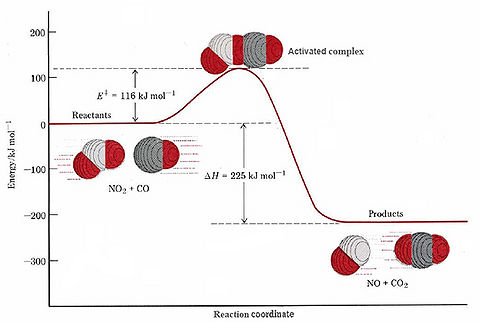
The same is true of our example of a bimolecular reaction. As the C end of a CO molecule approaches one of the O’s in NO₂, the electron clouds surrounding the molecules begin to repel each other and the energy of the system rises. This is shown in Figure \(\PageIndex{3}\). Only if the total energy of the two molecules exceeds the 116 kJ mol^–1 activation energy can they squeeze close enough together for a C—C bond to start to form. As this occurs the N—O bond begins to break, so that the activated complex has the structure

The dashed lines indicate bonds which are just beginning to form or are in the process of breaking. As the reaction occurs, the N—O bond lengthens and the O—C distance continually gets shorter. Consequently the difference between the N—O bond length and the C—O bond length (r_N—O – r_C—O) becomes larger and larger during the reaction. This difference, then, makes a convenient reaction coordinate.

Figure \(\PageIndex{3}\) Energy profile for the reaction between NO₂ and CO. As the two molecules approach closely, energy is needed to squeeze them together against the mutual repulsion of their outer electrons until the C atom and an O atom are close enough to a bond. If the two colliding molecules do not have at least 116 kJ mol^–1 between them, the O atom cannot be forced close enough to the C atom to transfer its allegiance from the N atom. The progress of a reaction like this is usually measured in terms of a convenient reaction coordinate, which in this case could be the N—O distance minus the C—O distance.