3.12: Diluting and Mixing Solutions
- Page ID
- 49285
\( \newcommand{\vecs}[1]{\overset { \scriptstyle \rightharpoonup} {\mathbf{#1}} } \)
\( \newcommand{\vecd}[1]{\overset{-\!-\!\rightharpoonup}{\vphantom{a}\smash {#1}}} \)
\( \newcommand{\id}{\mathrm{id}}\) \( \newcommand{\Span}{\mathrm{span}}\)
( \newcommand{\kernel}{\mathrm{null}\,}\) \( \newcommand{\range}{\mathrm{range}\,}\)
\( \newcommand{\RealPart}{\mathrm{Re}}\) \( \newcommand{\ImaginaryPart}{\mathrm{Im}}\)
\( \newcommand{\Argument}{\mathrm{Arg}}\) \( \newcommand{\norm}[1]{\| #1 \|}\)
\( \newcommand{\inner}[2]{\langle #1, #2 \rangle}\)
\( \newcommand{\Span}{\mathrm{span}}\)
\( \newcommand{\id}{\mathrm{id}}\)
\( \newcommand{\Span}{\mathrm{span}}\)
\( \newcommand{\kernel}{\mathrm{null}\,}\)
\( \newcommand{\range}{\mathrm{range}\,}\)
\( \newcommand{\RealPart}{\mathrm{Re}}\)
\( \newcommand{\ImaginaryPart}{\mathrm{Im}}\)
\( \newcommand{\Argument}{\mathrm{Arg}}\)
\( \newcommand{\norm}[1]{\| #1 \|}\)
\( \newcommand{\inner}[2]{\langle #1, #2 \rangle}\)
\( \newcommand{\Span}{\mathrm{span}}\) \( \newcommand{\AA}{\unicode[.8,0]{x212B}}\)
\( \newcommand{\vectorA}[1]{\vec{#1}} % arrow\)
\( \newcommand{\vectorAt}[1]{\vec{\text{#1}}} % arrow\)
\( \newcommand{\vectorB}[1]{\overset { \scriptstyle \rightharpoonup} {\mathbf{#1}} } \)
\( \newcommand{\vectorC}[1]{\textbf{#1}} \)
\( \newcommand{\vectorD}[1]{\overrightarrow{#1}} \)
\( \newcommand{\vectorDt}[1]{\overrightarrow{\text{#1}}} \)
\( \newcommand{\vectE}[1]{\overset{-\!-\!\rightharpoonup}{\vphantom{a}\smash{\mathbf {#1}}}} \)
\( \newcommand{\vecs}[1]{\overset { \scriptstyle \rightharpoonup} {\mathbf{#1}} } \)
\( \newcommand{\vecd}[1]{\overset{-\!-\!\rightharpoonup}{\vphantom{a}\smash {#1}}} \)
\(\newcommand{\avec}{\mathbf a}\) \(\newcommand{\bvec}{\mathbf b}\) \(\newcommand{\cvec}{\mathbf c}\) \(\newcommand{\dvec}{\mathbf d}\) \(\newcommand{\dtil}{\widetilde{\mathbf d}}\) \(\newcommand{\evec}{\mathbf e}\) \(\newcommand{\fvec}{\mathbf f}\) \(\newcommand{\nvec}{\mathbf n}\) \(\newcommand{\pvec}{\mathbf p}\) \(\newcommand{\qvec}{\mathbf q}\) \(\newcommand{\svec}{\mathbf s}\) \(\newcommand{\tvec}{\mathbf t}\) \(\newcommand{\uvec}{\mathbf u}\) \(\newcommand{\vvec}{\mathbf v}\) \(\newcommand{\wvec}{\mathbf w}\) \(\newcommand{\xvec}{\mathbf x}\) \(\newcommand{\yvec}{\mathbf y}\) \(\newcommand{\zvec}{\mathbf z}\) \(\newcommand{\rvec}{\mathbf r}\) \(\newcommand{\mvec}{\mathbf m}\) \(\newcommand{\zerovec}{\mathbf 0}\) \(\newcommand{\onevec}{\mathbf 1}\) \(\newcommand{\real}{\mathbb R}\) \(\newcommand{\twovec}[2]{\left[\begin{array}{r}#1 \\ #2 \end{array}\right]}\) \(\newcommand{\ctwovec}[2]{\left[\begin{array}{c}#1 \\ #2 \end{array}\right]}\) \(\newcommand{\threevec}[3]{\left[\begin{array}{r}#1 \\ #2 \\ #3 \end{array}\right]}\) \(\newcommand{\cthreevec}[3]{\left[\begin{array}{c}#1 \\ #2 \\ #3 \end{array}\right]}\) \(\newcommand{\fourvec}[4]{\left[\begin{array}{r}#1 \\ #2 \\ #3 \\ #4 \end{array}\right]}\) \(\newcommand{\cfourvec}[4]{\left[\begin{array}{c}#1 \\ #2 \\ #3 \\ #4 \end{array}\right]}\) \(\newcommand{\fivevec}[5]{\left[\begin{array}{r}#1 \\ #2 \\ #3 \\ #4 \\ #5 \\ \end{array}\right]}\) \(\newcommand{\cfivevec}[5]{\left[\begin{array}{c}#1 \\ #2 \\ #3 \\ #4 \\ #5 \\ \end{array}\right]}\) \(\newcommand{\mattwo}[4]{\left[\begin{array}{rr}#1 \amp #2 \\ #3 \amp #4 \\ \end{array}\right]}\) \(\newcommand{\laspan}[1]{\text{Span}\{#1\}}\) \(\newcommand{\bcal}{\cal B}\) \(\newcommand{\ccal}{\cal C}\) \(\newcommand{\scal}{\cal S}\) \(\newcommand{\wcal}{\cal W}\) \(\newcommand{\ecal}{\cal E}\) \(\newcommand{\coords}[2]{\left\{#1\right\}_{#2}}\) \(\newcommand{\gray}[1]{\color{gray}{#1}}\) \(\newcommand{\lgray}[1]{\color{lightgray}{#1}}\) \(\newcommand{\rank}{\operatorname{rank}}\) \(\newcommand{\row}{\text{Row}}\) \(\newcommand{\col}{\text{Col}}\) \(\renewcommand{\row}{\text{Row}}\) \(\newcommand{\nul}{\text{Nul}}\) \(\newcommand{\var}{\text{Var}}\) \(\newcommand{\corr}{\text{corr}}\) \(\newcommand{\len}[1]{\left|#1\right|}\) \(\newcommand{\bbar}{\overline{\bvec}}\) \(\newcommand{\bhat}{\widehat{\bvec}}\) \(\newcommand{\bperp}{\bvec^\perp}\) \(\newcommand{\xhat}{\widehat{\xvec}}\) \(\newcommand{\vhat}{\widehat{\vvec}}\) \(\newcommand{\uhat}{\widehat{\uvec}}\) \(\newcommand{\what}{\widehat{\wvec}}\) \(\newcommand{\Sighat}{\widehat{\Sigma}}\) \(\newcommand{\lt}{<}\) \(\newcommand{\gt}{>}\) \(\newcommand{\amp}{&}\) \(\definecolor{fillinmathshade}{gray}{0.9}\)|
How to Dilute a Solution by CarolinaBiological |

|
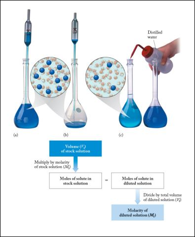
Often it is convenient to prepare a series of solutions of known concentrations by first preparing a single stock solution as described in Example 1 from Solution Concentrations. Aliquots (carefully measured volumes) of the stock solution can then be diluted to any desired volume. In other cases it may be inconvenient to weigh accurately a small enough mass of sample to prepare a small volume of a dilute solution. Each of these situations requires that a solution be diluted to obtain the desired concentration.
A pipet is used to measure 50.0 ml of 0.1027 M HCl into a 250.00-ml volumetric flask. Distilled water is carefully added up to the mark on the flask. What is the concentration of the diluted solution?
Solution
To calculate concentration, we first obtain the amount of HCI in the 50.0 ml (50.0 cm3) of solution added to the volumetric flask:
\[n_{\text{HCl}}=\text{50}\text{.0 cm}^{\text{3}}\text{ }\times \text{ }\dfrac{\text{0}\text{.1027 mmol}}{\text{1 cm}^{\text{3}}}=\text{5}\text{.14 mmol} \nonumber \]
Dividing by the new volume gives the concentration
\[c_{\text{HCl}}=\dfrac{n_{\text{HCl}}}{V}=\dfrac{\text{5}\text{.14 mmol}}{\text{250}\text{.00 cm}^{\text{3}}}=\text{0.0205 mmol cm}^{\text{-3}} \nonumber \]
Thus the new solution is 0.0205 M.
Alternatively,
\[n_{\text{HCl}}=\text{50}\text{.0 mL} ~\times~ \dfrac{\text{10}^{-3}\text{L}}{\text{1 ml}} ~\times~\dfrac{\text{0}\text{.1027 mol}}{\text{1 L}} \nonumber \]
\[~=~\text{5.14}\times{10}^{-3}\text{mol} \nonumber \]
\[c_{\text{HCl}}=\dfrac{n_{\text{HCl}}}{V} ~ = ~ \dfrac{\text{5}\text{.14}\times\text{10}^{-3}\text{mol}}{\text{250.00 ml}~\times~\dfrac{1 \text{ml}}{\text{10}^{-3}\text{L}}} \nonumber \]
\[~ = ~ \text{0.0205 mol/L} \nonumber \]
What volume of the solution of 0.316 46 M KI prepared in Example 1 from Solution Concentrations would be required to make 50.00 ml of 0.0500 M KI?
Solution
Using the volume and concentration of the desired solution, we can calculate the amount of KI required. Then the concentration of the original solution (0.316 46 M) can be used to convert that amount of KI to the necessary volume. Schematically
\[\begin{align} & V_{\text{new}}\xrightarrow{c_{\text{new}}}n_{\text{KI}}\xrightarrow{c_{\text{old}}}V_{\text{old}} \\ & \\ & V_{\text{old}}=\text{50}\text{.00 cm}^{\text{3}}\text{ }\times \text{ }\dfrac{\text{0}\text{.0500 mmol}}{\text{1 cm}^{\text{3}}}\text{ }\times \text{ }\dfrac{\text{1 cm}^{\text{3}}}{\text{0}\text{.316 46 mmol}}\text{ }=\text{7}\text{.90 cm}^{\text{3}} \\ \end{align} \nonumber \]
Thus we should dilute a 7.90-ml aliquot of the stock solution to 50.00 ml. This could be done by measuring 7.90 ml from a buret into a 50.00-ml volumetric flask and adding water up to the mark.
Note that the calculation above can be simplified, since the concentration and volume of a concentrated solution (Cconc and Vconc) were used to calculate the amount of solute, and this amount was entirely transferred to the dilute solution:
\[ C_{conc} \times V_{conc} = n_{conc} = n_{dil} = C_{dil} \times V_{dil} \nonumber \]
So
\[ C_{conc} \times V_{conc} = C_{dil} \times V_{dil} \nonumber \]
So for Example \(\PageIndex{2}\),
\[( 0.316 46 M ) \times (V_{conc}) = (50.00 \text{ ml} ) \times ( 0.0500 M) \nonumber \]
\[ V_{conc} = 7.90 \text{ mL} \nonumber \] , which will be diluted to 50.00 mL as before.
Note that the calculated volume will have the same dimensions as the input volume, and dimensional analysis tells us that in this case we don't need to convert to liters, since L cancels when we divide M (mol/L) by M (mol/L).


