3.5: Analysis of Compounds
- Page ID
- 49273
\( \newcommand{\vecs}[1]{\overset { \scriptstyle \rightharpoonup} {\mathbf{#1}} } \)
\( \newcommand{\vecd}[1]{\overset{-\!-\!\rightharpoonup}{\vphantom{a}\smash {#1}}} \)
\( \newcommand{\id}{\mathrm{id}}\) \( \newcommand{\Span}{\mathrm{span}}\)
( \newcommand{\kernel}{\mathrm{null}\,}\) \( \newcommand{\range}{\mathrm{range}\,}\)
\( \newcommand{\RealPart}{\mathrm{Re}}\) \( \newcommand{\ImaginaryPart}{\mathrm{Im}}\)
\( \newcommand{\Argument}{\mathrm{Arg}}\) \( \newcommand{\norm}[1]{\| #1 \|}\)
\( \newcommand{\inner}[2]{\langle #1, #2 \rangle}\)
\( \newcommand{\Span}{\mathrm{span}}\)
\( \newcommand{\id}{\mathrm{id}}\)
\( \newcommand{\Span}{\mathrm{span}}\)
\( \newcommand{\kernel}{\mathrm{null}\,}\)
\( \newcommand{\range}{\mathrm{range}\,}\)
\( \newcommand{\RealPart}{\mathrm{Re}}\)
\( \newcommand{\ImaginaryPart}{\mathrm{Im}}\)
\( \newcommand{\Argument}{\mathrm{Arg}}\)
\( \newcommand{\norm}[1]{\| #1 \|}\)
\( \newcommand{\inner}[2]{\langle #1, #2 \rangle}\)
\( \newcommand{\Span}{\mathrm{span}}\) \( \newcommand{\AA}{\unicode[.8,0]{x212B}}\)
\( \newcommand{\vectorA}[1]{\vec{#1}} % arrow\)
\( \newcommand{\vectorAt}[1]{\vec{\text{#1}}} % arrow\)
\( \newcommand{\vectorB}[1]{\overset { \scriptstyle \rightharpoonup} {\mathbf{#1}} } \)
\( \newcommand{\vectorC}[1]{\textbf{#1}} \)
\( \newcommand{\vectorD}[1]{\overrightarrow{#1}} \)
\( \newcommand{\vectorDt}[1]{\overrightarrow{\text{#1}}} \)
\( \newcommand{\vectE}[1]{\overset{-\!-\!\rightharpoonup}{\vphantom{a}\smash{\mathbf {#1}}}} \)
\( \newcommand{\vecs}[1]{\overset { \scriptstyle \rightharpoonup} {\mathbf{#1}} } \)
\( \newcommand{\vecd}[1]{\overset{-\!-\!\rightharpoonup}{\vphantom{a}\smash {#1}}} \)
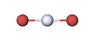
\(\newcommand{\avec}{\mathbf a}\) \(\newcommand{\bvec}{\mathbf b}\) \(\newcommand{\cvec}{\mathbf c}\) \(\newcommand{\dvec}{\mathbf d}\) \(\newcommand{\dtil}{\widetilde{\mathbf d}}\) \(\newcommand{\evec}{\mathbf e}\) \(\newcommand{\fvec}{\mathbf f}\) \(\newcommand{\nvec}{\mathbf n}\) \(\newcommand{\pvec}{\mathbf p}\) \(\newcommand{\qvec}{\mathbf q}\) \(\newcommand{\svec}{\mathbf s}\) \(\newcommand{\tvec}{\mathbf t}\) \(\newcommand{\uvec}{\mathbf u}\) \(\newcommand{\vvec}{\mathbf v}\) \(\newcommand{\wvec}{\mathbf w}\) \(\newcommand{\xvec}{\mathbf x}\) \(\newcommand{\yvec}{\mathbf y}\) \(\newcommand{\zvec}{\mathbf z}\) \(\newcommand{\rvec}{\mathbf r}\) \(\newcommand{\mvec}{\mathbf m}\) \(\newcommand{\zerovec}{\mathbf 0}\) \(\newcommand{\onevec}{\mathbf 1}\) \(\newcommand{\real}{\mathbb R}\) \(\newcommand{\twovec}[2]{\left[\begin{array}{r}#1 \\ #2 \end{array}\right]}\) \(\newcommand{\ctwovec}[2]{\left[\begin{array}{c}#1 \\ #2 \end{array}\right]}\) \(\newcommand{\threevec}[3]{\left[\begin{array}{r}#1 \\ #2 \\ #3 \end{array}\right]}\) \(\newcommand{\cthreevec}[3]{\left[\begin{array}{c}#1 \\ #2 \\ #3 \end{array}\right]}\) \(\newcommand{\fourvec}[4]{\left[\begin{array}{r}#1 \\ #2 \\ #3 \\ #4 \end{array}\right]}\) \(\newcommand{\cfourvec}[4]{\left[\begin{array}{c}#1 \\ #2 \\ #3 \\ #4 \end{array}\right]}\) \(\newcommand{\fivevec}[5]{\left[\begin{array}{r}#1 \\ #2 \\ #3 \\ #4 \\ #5 \\ \end{array}\right]}\) \(\newcommand{\cfivevec}[5]{\left[\begin{array}{c}#1 \\ #2 \\ #3 \\ #4 \\ #5 \\ \end{array}\right]}\) \(\newcommand{\mattwo}[4]{\left[\begin{array}{rr}#1 \amp #2 \\ #3 \amp #4 \\ \end{array}\right]}\) \(\newcommand{\laspan}[1]{\text{Span}\{#1\}}\) \(\newcommand{\bcal}{\cal B}\) \(\newcommand{\ccal}{\cal C}\) \(\newcommand{\scal}{\cal S}\) \(\newcommand{\wcal}{\cal W}\) \(\newcommand{\ecal}{\cal E}\) \(\newcommand{\coords}[2]{\left\{#1\right\}_{#2}}\) \(\newcommand{\gray}[1]{\color{gray}{#1}}\) \(\newcommand{\lgray}[1]{\color{lightgray}{#1}}\) \(\newcommand{\rank}{\operatorname{rank}}\) \(\newcommand{\row}{\text{Row}}\) \(\newcommand{\col}{\text{Col}}\) \(\renewcommand{\row}{\text{Row}}\) \(\newcommand{\nul}{\text{Nul}}\) \(\newcommand{\var}{\text{Var}}\) \(\newcommand{\corr}{\text{corr}}\) \(\newcommand{\len}[1]{\left|#1\right|}\) \(\newcommand{\bbar}{\overline{\bvec}}\) \(\newcommand{\bhat}{\widehat{\bvec}}\) \(\newcommand{\bperp}{\bvec^\perp}\) \(\newcommand{\xhat}{\widehat{\xvec}}\) \(\newcommand{\vhat}{\widehat{\vvec}}\) \(\newcommand{\uhat}{\widehat{\uvec}}\) \(\newcommand{\what}{\widehat{\wvec}}\) \(\newcommand{\Sighat}{\widehat{\Sigma}}\) \(\newcommand{\lt}{<}\) \(\newcommand{\gt}{>}\) \(\newcommand{\amp}{&}\) \(\definecolor{fillinmathshade}{gray}{0.9}\)Up to this point we have obtained all stoichiometric ratios from the coefficients of balanced chemical equations. Chemical formulas also indicate relative amounts of substance, however, and stoichiometric ratios may be derived from them, too. For example, the formula HgBr2 tells us that no matter how large a sample of mercuric bromide we have, there will always be 2 mol of bromine atoms for each mole of mercury atoms. That is, from the formula HgBr2 and the submicroscopic image below, we have the stoichiometric ratio

\[ \text{S}\left( \frac{\text{Br}}{\text{Hg}} \right)=\frac{\text{2 mol Br}}{\text{1 mol Hg}}\label{1} \]
We could also determine that for HgBr2
\[ \text{S}\left( \frac{\text{Hg}}{\text{HgBr}_{\text{2}}} \right)=\frac{\text{1 mol Hg}}{\text{1 mol HgBr}_{\text{2}}} \nonumber \]
\[ \text{S}\left( \frac{\text{Br}}{\text{HgBr}_{\text{2}}} \right)=\text{ }\frac{\text{2 mol Br}}{\text{1 mol HgBr}_{\text{2}}} \nonumber \]
(The reciprocals of these stoichiometric ratios are also valid for HgBr2.)
Stoichiometric ratios derived from formulas instead of equations are involved in the most common procedure for determining the empirical formulas of compounds which contain only C, H, and O. The process is depicted in the image below for reference. A weighed quantity of the substance to be analyzed is placed in a combustion train and heated in a stream of dry O2. All the H in the compound is converted to H2O(g) which is trapped selectively in a previously weighed absorption tube. All the C is converted to CO2(g) and this is absorbed selectively in a second tube. The increase of mass of each tube tells, respectively, how much H2O and CO2 were produced by combustion of the sample.

A 6.49-mg sample of ascorbic acid (vitamin C) was burned in a combustion train. 9.74 mg CO2 and 2.64 mg H2O were formed. Determine the empirical formula of ascorbic acid.
Solution
We need to know the amount of C, the amount of H, and the amount of O in the sample. The ratio of these gives the subscripts in the formula. The first two may be obtained from the masses of CO2 and H2O using the molar masses and the stoichiometric ratios
\[ \text{S}\left( \frac{\text{C}}{\text{CO}_{\text{2}}} \right)=\frac{\text{1 mol C}}{\text{1 mol CO}_{\text{2}}} \nonumber \]
\[ \text{S}\left( \frac{\text{H}}{\text{H}_{\text{2}}\text{O}} \right)=\frac{\text{2 mol H}}{\text{1 mol H}_{\text{2}}\text{O}} \nonumber \]
Thus
\[\begin{align*} n_{\text{C}}&=\text{9}\text{.74}\times \text{10}^{\text{-3}}\text{g CO}_{\text{2}}\times {\frac{\text{1 mol CO}_{\text{2}}}{\text{44}\text{.01 g CO}_{\text{2}}}} \times {\frac{\text{1 mol C}}{\text{1 mol CO}_{\text{2}}}} = \text{2.21}\times \text{10}^{-4}\text{ mol C}\\ { } \\ n_{\text{H}} &=\text{2}\text{.64}\times \text{10}^{\text{-3}}\text{g H}_{\text{2}}\text{O}\times {\frac{\text{1 mol H}_{\text{2}}\text{O}}{\text{18}\text{.02 g H}_{\text{2}}\text{O}}} \times {\frac{\text{2 mol H}}{\text{1 mol H}_{\text{2}}\text{O}}} = \text{2.93}\times \text{10}^{\text{-4}}\text{ mol H} \end{align*} \nonumber \]
The compound may also have contained oxygen. To see if it does, calculate the masses of C and H and subtract from the total mass of sample
\[\begin{align*} m_{\text{C}}&=\text{2}\text{.21}\times \text{10}^{\text{-4}}\text{ mol C}\times \frac{\text{12}\text{.01 g C}}{\text{1 mol C}}=\text{2}\text{.65}\times \text{10}^{\text{-3}}\text{g C}=\text{2}\text{.65 mg C} \\ & \\ m_{\text{H}}&=\text{2}\text{.93}\times \text{10}^{\text{-4}}\text{ mol H}\times \frac{\text{1}\text{.008 g H}}{\text{1 mol H}}=\text{2}\text{.95}\times \text{10}^{\text{-4}}\text{g H}=\text{0}\text{0.295 mg H} \\ \end{align*} \nonumber \]
Thus we have
\[6.49 \text{mg sample} – 2.65 \text{mg C} – 0.295 \text{mg H} = 3.54 \text{mg O} \nonumber \]
and
\[ n_{\text{O}}=\text{3}\text{.54}\times \text{10}^{\text{-3}}\text{ g O}\times {\frac{\text{1 mol O}}{\text{16.00 g O}}} =\text{2}\text{.21}\times \text{10}^{\text{-4}}\text{ mol O} \nonumber \]
The ratios of the amounts of the elements in ascorbic acid are therefore
\[ {\frac{n_{\text{H}}}{n_{\text{C}}}=\frac{\text{2}\text{.93}\times \text{10}^{\text{-4}}\text{ mol H}}{\text{2}\text{.21}\times \text{10}^{\text{-4}}\text{ mol C}}=\frac{\text{1}\text{.33 mol H}}{\text{1 mol C}}=\frac{\text{1}\tfrac{1}{3}\text{mol H}}{\text{1 mol C}}=\frac{\text{4 mol H}}{\text{3 mol C}}} \nonumber \]
\[ {\frac{n_{\text{O}}}{n_{\text{C}}}=\frac{\text{2}\text{.21}\times \text{10}^{\text{-4}}\text{ mol O}}{\text{2}\text{.21}\times \text{10}^{\text{-4}}\text{ mol C}}=\frac{\text{1 mol O}}{\text{1 mol C}}=\frac{\text{3 mol O}}{\text{3 mol C}}} \nonumber \]
Since nC:nH:nO is 3 mol C:4 mol H:3 mol O, the empirical formula is C3H4O3.
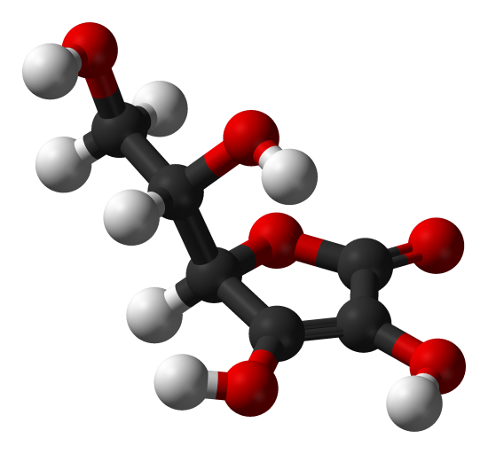
A drawing of a molecule of ascorbic acid is shown here. You can determine by counting the atoms that the molecular formula is C6H8O6—exactly double the empirical formula. It is also evident that there is more to know about a molecule than just how many atoms of each kind are present. In ascorbic acid, as in other molecules, the way the atoms are connected together and their arrangement in three-dimensional space are quite important. A picture showing which atoms are connected to which is called a structural formula. Empirical formulas may be obtained from percent composition or combustion-train experiments, and, if the molecular weight is known, molecular formulas may be determined from the same data. More complicated experiments are required to find structural formulas. In Example 2 we obtained the mass of O by subtracting the masses of C and H from the total mass of sample. This assumed that only C, H, and O were present. Sometimes such an assumption may be incorrect. When penicillin was first isolated and analyzed, the fact that it contained sulfur was missed. This mistake was not discovered for some time because the atomic weight of sulfur is almost exactly twice that of oxygen. Two atoms of oxygen were substituted in place of one sulfur atom in the formula.
A 3D representation of L-Ascorbic Acid


