7.7: Solutions for Selected Problems

Exercise 7.2.1:

Exercise 7.2.2:

Exercise 6.2.3:

a) Iron charges: \(Fe(II) + Fe(III) = 5^{+}\)

Ligand charges: \(2 \: sulfides \: = 2 \times 2^{-} = 4^{-} ; 4 \: cysteines \: = 4 \times 1^{-} = 4^{-} ; \: total \:= 8^{-}\)

Overall: 3^-

b) Iron charges: \(2 \times Fe(II) + Fe(III) = 4^{+} + 3^{+} = 7^{+}\)

Ligand charges: \(4 \: sulfides \: = 4 \times 2^{-} = 8^{-}; 3 \: cysteines \: = 3 \times 1^{-} = 3^{-} ; \: total \: = 11^{-}\)

Overall: 4^-

c) Iron charges: \(3 \times Fe(II) + Fe(III) = 6^{+} + 3^{+} = 9^{+}\)

Ligand charges: \(4 \: sulfides \: = 4 \times 2^{-} = 8^{-} ; 4 \: cysteines \: = 4 \times 1^{-} = 4^{-} ; \: total \: = 12^{-}\)

Overall: 3^-

Exercise 7.2.4:

Upon reduction, the charge on a 2Fe2S cluster will increase from 3^- to 4^-, assuming it starts in a mixed Fe(II)/(III) state (whereas if it starts in a Fe(III)/(III) state, the overall charge will increase from 2^- to 3^-). These anions would be stabilised by strong intermolecular interactions such as ion-dipole forces. Both states (oxidised and reduced) will be stabilised by a polar environment, but the more highly charged reduced state will depend even more strongly on stabilisation by the environment. As a result, we might expect the reduction potential to be lower when surrounded by nonpolar amino acid residues, and higher if surrounded by polar residues.

Exercise 7.2.5:

Exercise 7.2.6:

Exercise 7.2.7:

Exercise 7.2.8:

Exercise 7.2.9:

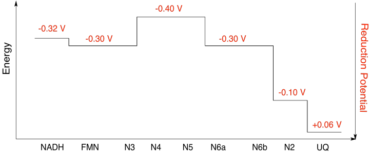
a) N1a and N1b are most likely not involved, because their reduction potentials are too negative.

b)

Exercise 7.2.10:

Assuming the reduction potentials are:

\[N5(ox) + e^{-} \rightarrow N5(red)\) \(E^{o}_{red}= -0.40V \nonumber\]

\[N6a(ox) + e^{-} \rightarrow N6a(red)\) \(E^{o}_{red} = -0.30V \nonumber\]

Then the potential difference for the reaction, \(\Delta E^{o} = -0.30 - (-0.40)V = 0.10V\)

The Faraday relation \(\Delta G= -n F \Delta E^{o} \) gives

\[\Delta G = -1 \times 96485 \frac{J}{V \: mol} \times 0.10 V = 9649 \frac{J}{mol} = 9.7 \frac{kJ}{mol} \nonumber\]

Exercise 7.3.1:

Heme b.

Exercise 7.3.2:

A porphyrin contains four pyrrole rings (five-membered, aromatic ring containing a nitrogen) arranged to form a 16-membered macrocycle.

Exercise 7.3.3:

Exercise 7.3.4:

Exercise 7.3.5:

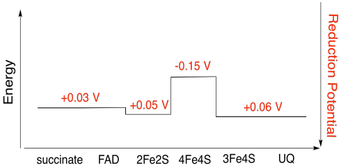
Assuming the reduction potentials are:

\[4Fe4s(ox) + e^{-} \rightarrow 4Fe4S(red)\) \(E^{o}_{red} = -0.15V \nonumber\]

\[3Fe4S(ox) + e^{-} \rightarrow 3Fe4S(red)\) \(E^{o}_{red} = 0.06V \nonumber\]

Then the potential difference for the reaction, \(\Delta E^{o} = 0.06 -(-0.15)V = 0.21V\)

The Faraday relation \(\Delta G = -n F \Dleta E^{o}\) gives

\[\Delta G = -1 \times 96485 \frac{J}{V \: mol} \times 0.21 V = 20262 \frac{J}{mol} = 20 \frac{kJ}{mol} \nonumber\]

Exercise 7.3.6:

a) Iron charges: \(2 \times Fe(III) = 6^{+}\)

Ligand charges: \(2 \: sulfides \: = 2 \times 2^{-}= 4^{-} ; 4 \: cysteines \: = 4 \times 1^{-} = 4^{-} ; \: total \: = 8^{-}\)

Overall: 2^-

b) Iron charges: \(3 \times Fe(III) = 9^{+}\)

Ligand charges: \(4 \: sulfides \: 4 \times 2^{-} = 8^{-} ; 3 \: cysteines \: = 3 \times 1^{-} = 3^{-} ; \: total \: = 11^{-}\)

Overall: 2^-

c) Iron charges: \(4 \times Fe(III) = 12^{+}\)

Ligand charges: \(4 \: sulfides = 4 \times 2^{-} = 8^{-} ; 4 \: cysteines \: = 4 \times 1^{-} = 4^{-} ; \: total \: = 12^{-}\)

Overall: 0

Exercise 7.4.1:

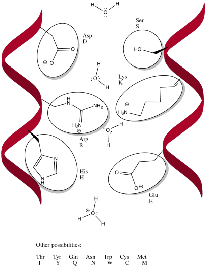
Arninine and lysine are positively charged at neutral pH.

Exercise 7.4.2:

Exercise 7.4.3:

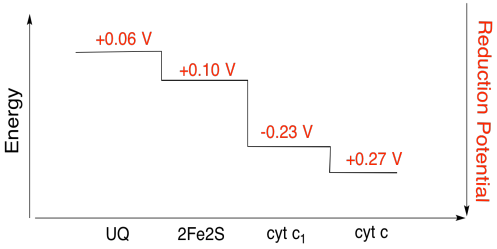
Assuming the reduction potentials are:

\[2Fe2S(ox) + e^{-} \rightarrow 2Fe2S(red)\) \(E^{o}_{red} = 0.10V \nonumber\]

\[cyt \: c_{1} (ox) + 3^{-} \rightarrow cyt \: c_{1} (red)\) \(E^{o}_{red}= 0.230V \nonumber\]

Then the potential difference for the reaction, \(\Delta E^{o} = 0.23- (0.10) V = 0.13V\)

The Faraday relation \(\Delta G = -nF \Delta E^{o}\) gives

\[\Delta G = -1 \times 96485 \frac{J}{V \: mol} \times 0.13V = 12543 \frac{J}{mol} = 12.5 \frac{kJ}{mol} \nonumber\]

Exercise 7.4.4:

The positive arginine residues would confer partial positive charge on the ubiquinone via hydrogen bonding; the ubiquinone would have a more positive reduction potential as a result.

Exercise 7.5.1:

\[\ce{O2 -> H2O} \nonumber\]

\(\ce{O2 -> 2H2O}\) (O balanced)

\(\ce{O2 + 4H^{+} -> 2H2O}\) (H balanced)

\(\ce{O2 + 4e^{-} + 4H^{+} -> 2H2O}\) (charge balanced)

Exercise 7.5.2:

Exercise 7.5.3:

Exercise 7.5.4:

a)

b) tetrahedral

c) Cu(I) = d¹⁰

4 donors = 8 e^-

total = 18e^-

d) 2 x Cu(I) = 2⁺

2 x Cys-S^- = 2^-

All others neutral

Total = 0

Exercise 7.5.5:

a)

) trigonal planar

c) Cu(I) = d¹⁰

3 donors = 6 e^-

total = 16 e^-

d) Cu(I) = 1⁺

histidines neutral

Total = 1⁺

Exercise 7.5.6:

Exercise 7.5.7:

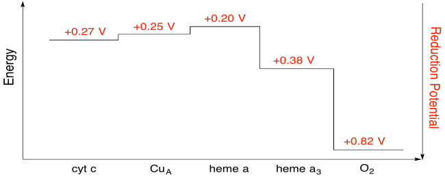
Assuming the reduction potentials are:

\[heme \: a(ox) + e^{-} \rightarrow heme \: a(red)\) \(E^{o}_{red} = 0.20V \nonumber\]

\[heme \: a_{3}(ox) + e^{-} \rightarrow heme \: a_{3}(red)\) \(E^{o}_{red} = 0.38V \nonumber\]

Then the potential difference for the reaction, \(\Delta E^{o} = 0.38 - (0.20)V = 0.18V\)

The Faraday relation \(\Delta G = -n F \Delta E^{o} \) gives

\[\Delta G = -1 \times 96485 \frac{J}{V \: mol} \times 0.13V = 17367 \frac{J}{mol} = 17.4 \frac{kJ}{mol} \nonumber\]

Exercise 7.6.1:

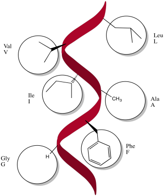
These amino acids would probably be non-polar: alanine, glycine, methionine, isoleucine, leucine, methionine, phenylalanine, tryptophan, valine.

Exercise 7.6.2:

There is always an equilibrium between the protonated state and the deprotonated state in a charged amino acid residue. For this position, an amino acid is needed that is more reliably in the protonated state; that is, the equilibrium lies more heavily to the protonated side of the equation. Because of the resonance-stabilised cation that results from protonation, arginine is much more likely to remain in a protonated state than lysine. That will make for a more efficient millwheel.

Exercise 7.6.3:

ADP and phosphate are both anions; they would repel normally each other. When bound in the active site, their charges are likely neutralized by complementary charges in the active site.

Exercise 7.6.4:

Assuming the reduction potentials are:

\[\ce{NAD^{+} + 2e^{-} + 2H^{+} -> NADH}\) \(E^{o}_{red} = -0.32V \nonumber\]

\[\ce{0.5 O2 + 2e^{-} + 2H^{+} -> H2O}\) \(E^{o}_{red} = 0.816V \nonumber\]

Then the potential difference for the reaction, \(\Delta E^{o} = 0.816 - (-0.32)V = 1.136V\)

The Faraday relation \(\Delta G = -NF \Delta E^{o}\) gives

\[\Delta G = -2 \times 96475 \frac {J}{V \: mol} \times 1.136V = 219213 \frac{J}{mol} = 219 \frac{kJ}{mol} \nonumber\]

so \(\frac{219 \frac{kJ}{mol}} {30 \frac{kJ}{mol}} = 7.3\)

With 100% efficiency, 7 moles of ATP could be produced per mole of NADH. In reality, about half that amount is produced (closer to 3 moles ATP per mole NADH).