23.2: Kramers’ Theory

In our treatment the motion of the reactant over the transition state was treated as a free transitional degree of freedom. This ballistic or inertial motion is not representative of dynamics in soft matter at room temperature. Kramers’ theory is the leading approach to describe diffusive barrier crossing. It accounts for friction and thermal agitation that reduce the fraction of successful barrier crossings. Again, the rates are obtained from the flux over barrier along reaction coordinate, Equation (23.1).

One approach is to treat diffusive crossing over the barrier in a potential using the Smoluchowski equation. The diffusive flux under influence of potential has two contributions:

1. Concentration gradient \(dC/dξ\). Proportional to diffusion coefficient, \(D\).
2. Force from gradient of potential.

\[ J(\xi)=-D \frac{d C(\xi)}{d \xi}-\frac{C(\xi)}{\zeta} \frac{d U(\xi)}{d \xi} \nonumber\]

As discussed earlier \(ζ\) is the friction coefficient and in one dimension:

\[ \zeta=\frac{k_{B} T}{D} \nonumber\]

Written in terms of a probability density \(P\)

\[\begin{align*} J &=D\left(-\frac{P}{k_{B} T} \frac{d U}{d \xi}-\frac{d P}{d \xi}\right) \\ &=-D e^{-U / k_{B} T} \frac{d}{d \xi}\left(P e^{U / k_{B} T}\right) \end{align*}\]

or

\[ J e^{U / k_{B} T}=-D \frac{d}{d \xi} P e^{U / k_{B} T} \]

Here we have assumed that \(D\) and \(ζ\) are not functions of \(ξ\).

The next important assumption of Kramers’ theory is that we can solve for the diffusive flux using the steady-state approximation. This allows us to set: \(J\) = constant. Integrate along \(ξ\) over barrier.

\[ \begin{align*} J \int_{a}^{b} e^{U / k_{B} T} d \xi * &=-D \int_{a}^{b} d P e^{U / k_{B} T} \\[4pt]  J \int_{a}^{b} e^{U(\xi) / k_{B} T} d \xi &=D\left\{P_{R} e^{U_{R} / k_{B} T}-P_{P} e^{U_{P} / k_{B} T}\right\} \end{align*}\]

\(P_i\) are the probabilities of occupying the \(R\) or \(P\) state, and \(U_i\) are the energies of the \(R\) and \(P\) states. The right hand side of this equation describes net flux across barrier.

Let’s consider only flux from \(R\longrightarrow P\): \( J_{R\longrightarrow P} \), which we do by setting \(P_P\longrightarrow 0\). This is just a barrier escape problem. Also as a reference point, we set \(U_R(ξ_R) = 0\).

\[ J_{R \rightarrow P}=\frac{D P_{R}}{\int_{a}^{b} e^{U(\xi) / k_{B} T} d \xi} \label{23.2.2}\]

The flux is linearly proportional to the diffusion coefficient and the probability of being in the reactant state. The flux is reduced by a factor that describes the energetic barrier to be overcome. Now let’s evaluate with a specific form of the potential. The simplest form is to model \(U(ξ)\) with parabolas. The reactant well is given by

\[ U_{R}=\frac{1}{2} m \omega_{R}^{2}\left(\xi-\xi_{R}\right)^{2} \label{23.2.3}\]

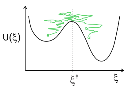
and we set \(\xi_R \longrightarrow 0\). The barrier is modeled by an inverted parabola centered at the transition state with a barrier height for the forward reaction \(E_f\) and a width given by the barrier frequency \(ω_{bar}\):

\[ U_{\mathrm{bar}}=E_{f}-\frac{1}{2} m \omega_{\mathrm{bar}}^{2}\left(\xi-\xi^{‡}\right)^{2} \nonumber\]

In essence this is treating the evolution of the probability distribution as the motion of a fictitious particle with mass \(m\).

First we evaluate the denominator in Equation \ref{23.2.2}. \(e^{U_{bar}/k_BT}\) is a probability density that is peaked at \( \xi^‡\), so changing the limits on the integral does not affect things much.

\[\int_{a}^{b} e^{U_{b a r} / k_{B} T} d \xi \approx \int_{-\infty}^{+\infty} d \xi \exp \left[-\frac{m \omega_{B}^{2}\left(\xi-\xi^{‡}\right)^{2}}{2 k_{B} T}\right]=\sqrt{\frac{2 \pi k_{B} T}{m \omega_{B}^{2}}} \nonumber\]

Then Equation \ref{23.2.2} becomes

\[ J_{R \rightarrow P}=\omega_{\text {bar }} D \sqrt{\frac{m}{2 \pi k_{B} T}} e^{-E_{f} / k_{B} T} P_{R} \label{23.2.4}\]

Next, let’s evaluate \(P_R\). For a the Gaussian well in Equation \ref{23.2.3}, the probability density along \(ξ\) is \(P_R = e^{-U_{R} / k_{B} T}\):

\[ P_{R}(\xi)=\exp \left[-\frac{1}{2} m \omega_{R}^{2}\left(\xi-\xi_{R}\right)^{2} / k_{B} T\right] \nonumber\]

\[ P_{R} \approx \int_{-\infty}^{+\infty} P_{R}(\xi) d \xi=\omega_{R} \sqrt{\frac{m}{2 \pi k_{B} T}} \nonumber\]

Substituting this into Equation \ref{23.2.4} we have

\[ J_{R \rightarrow P}=\omega_{R} \omega_{b a r} D\left(\frac{m}{2 \pi k_{B} T}\right) e^{-E_{f} / k_{B} T} \nonumber\]

Using the Einstein relation \( D = k_BT/\zeta \), we find that the forward flux scales inversely with friction (or viscosity).

\[ J_{R \rightarrow P}=\frac{\omega_{R}}{2 \pi} \frac{\omega_{b a r}}{\zeta} e^{-E_{f} / k_{B} T} \]

Also, the factor of \(m\) disappears when the problem is expressed in mass-weighted coordinates \(\omega_{\text {bar }}=\sqrt{m} \omega_{\text {bar }}\). Note the similarity of Equation (9) to transition state theory. If we associate the period of the particle in the reactant well with the barrier crossing frequency,

\[ \frac{\omega_{R}}{2 \pi} \Rightarrow v=\frac{k_{B} T}{h} \nonumber\]

then we can also find that we an expression for the transmission coefficient in this model:

\[ k_{diff}=\kappa_{diff} k_{TST} \nonumber\]

\[ \kappa_{diff}=\dfrac{\omega_{bar}}{\zeta}\ll 1 \nonumber\]

This is the reaction rate in the strong damping, or diffusive, limit. Hendrik Kramers actually solved a more general problem based on the Fokker–Planck Equation that described intermediate to strong damping. The reaction rate was described as

\[ k_{Kr}=\kappa_{Kr} k_{TST} \nonumber\]

\[\kappa_{K r}=\frac{1}{\omega_{b a r}}\left(-\frac{\zeta}{2}+\sqrt{\frac{\zeta^{2}}{4}+\omega_{b a r}^{2}}\right) \nonumber\]

\[ \zeta=\frac{1}{m k_{B} T} \int_{0}^{\infty} d t\langle\xi(0) \xi(t)\rangle \nonumber\]

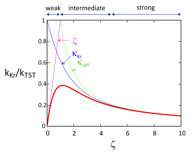
This shows a crossover in behavior between the strong damping (or diffusive) behavior described above and an intermediate damping regime:

• Strong damping/friction: \(\zeta \longrightarrow \infty\) \(\kappa_{Kr}\longrightarrow\dfrac{\omega_{bar}}{\zeta} \nonumber\)
• Intermediate damping: \(\zeta <<2\omega_B\) \(\kappa_{Kr}\longrightarrow 1\) and \(k_{Kr}\longrightarrow k_{TST} \nonumber\)

In the weak friction limit, Kramers argued that the reaction rate scaled as

\[k_{\text {weak }} \sim \zeta k_{T S T} \nonumber\]

That is, if you had no friction at all, the particle would just move back and forth between the reactant and product state without committing to a particular well. You need some dissipation to relax irreversibly into the product well. On the basis of this we expect an optimal friction that maximizes \(κ\), which balances the need for some dissipation but without so much that barrier crossing is exceedingly rare. This “Kramers turnover” is captured by the interpolation formula

\[\kappa^{-1}=\kappa_{K r}^{-1}+\kappa_{\text {weak }}^{-1} \nonumber\]