
23.1: Transition State Theory
- Page ID
- 294374

\( \newcommand{\vecs}[1]{\overset { \scriptstyle \rightharpoonup} {\mathbf{#1}} } \)
\( \newcommand{\vecd}[1]{\overset{-\!-\!\rightharpoonup}{\vphantom{a}\smash {#1}}} \)
\( \newcommand{\id}{\mathrm{id}}\) \( \newcommand{\Span}{\mathrm{span}}\)
( \newcommand{\kernel}{\mathrm{null}\,}\) \( \newcommand{\range}{\mathrm{range}\,}\)
\( \newcommand{\RealPart}{\mathrm{Re}}\) \( \newcommand{\ImaginaryPart}{\mathrm{Im}}\)
\( \newcommand{\Argument}{\mathrm{Arg}}\) \( \newcommand{\norm}[1]{\| #1 \|}\)
\( \newcommand{\inner}[2]{\langle #1, #2 \rangle}\)
\( \newcommand{\Span}{\mathrm{span}}\)
\( \newcommand{\id}{\mathrm{id}}\)
\( \newcommand{\Span}{\mathrm{span}}\)
\( \newcommand{\kernel}{\mathrm{null}\,}\)
\( \newcommand{\range}{\mathrm{range}\,}\)
\( \newcommand{\RealPart}{\mathrm{Re}}\)
\( \newcommand{\ImaginaryPart}{\mathrm{Im}}\)
\( \newcommand{\Argument}{\mathrm{Arg}}\)
\( \newcommand{\norm}[1]{\| #1 \|}\)
\( \newcommand{\inner}[2]{\langle #1, #2 \rangle}\)
\( \newcommand{\Span}{\mathrm{span}}\) \( \newcommand{\AA}{\unicode[.8,0]{x212B}}\)
\( \newcommand{\vectorA}[1]{\vec{#1}} % arrow\)
\( \newcommand{\vectorAt}[1]{\vec{\text{#1}}} % arrow\)
\( \newcommand{\vectorB}[1]{\overset { \scriptstyle \rightharpoonup} {\mathbf{#1}} } \)
\( \newcommand{\vectorC}[1]{\textbf{#1}} \)
\( \newcommand{\vectorD}[1]{\overrightarrow{#1}} \)
\( \newcommand{\vectorDt}[1]{\overrightarrow{\text{#1}}} \)
\( \newcommand{\vectE}[1]{\overset{-\!-\!\rightharpoonup}{\vphantom{a}\smash{\mathbf {#1}}}} \)
\( \newcommand{\vecs}[1]{\overset { \scriptstyle \rightharpoonup} {\mathbf{#1}} } \)
\( \newcommand{\vecd}[1]{\overset{-\!-\!\rightharpoonup}{\vphantom{a}\smash {#1}}} \)
\(\newcommand{\avec}{\mathbf a}\) \(\newcommand{\bvec}{\mathbf b}\) \(\newcommand{\cvec}{\mathbf c}\) \(\newcommand{\dvec}{\mathbf d}\) \(\newcommand{\dtil}{\widetilde{\mathbf d}}\) \(\newcommand{\evec}{\mathbf e}\) \(\newcommand{\fvec}{\mathbf f}\) \(\newcommand{\nvec}{\mathbf n}\) \(\newcommand{\pvec}{\mathbf p}\) \(\newcommand{\qvec}{\mathbf q}\) \(\newcommand{\svec}{\mathbf s}\) \(\newcommand{\tvec}{\mathbf t}\) \(\newcommand{\uvec}{\mathbf u}\) \(\newcommand{\vvec}{\mathbf v}\) \(\newcommand{\wvec}{\mathbf w}\) \(\newcommand{\xvec}{\mathbf x}\) \(\newcommand{\yvec}{\mathbf y}\) \(\newcommand{\zvec}{\mathbf z}\) \(\newcommand{\rvec}{\mathbf r}\) \(\newcommand{\mvec}{\mathbf m}\) \(\newcommand{\zerovec}{\mathbf 0}\) \(\newcommand{\onevec}{\mathbf 1}\) \(\newcommand{\real}{\mathbb R}\) \(\newcommand{\twovec}[2]{\left[\begin{array}{r}#1 \\ #2 \end{array}\right]}\) \(\newcommand{\ctwovec}[2]{\left[\begin{array}{c}#1 \\ #2 \end{array}\right]}\) \(\newcommand{\threevec}[3]{\left[\begin{array}{r}#1 \\ #2 \\ #3 \end{array}\right]}\) \(\newcommand{\cthreevec}[3]{\left[\begin{array}{c}#1 \\ #2 \\ #3 \end{array}\right]}\) \(\newcommand{\fourvec}[4]{\left[\begin{array}{r}#1 \\ #2 \\ #3 \\ #4 \end{array}\right]}\) \(\newcommand{\cfourvec}[4]{\left[\begin{array}{c}#1 \\ #2 \\ #3 \\ #4 \end{array}\right]}\) \(\newcommand{\fivevec}[5]{\left[\begin{array}{r}#1 \\ #2 \\ #3 \\ #4 \\ #5 \\ \end{array}\right]}\) \(\newcommand{\cfivevec}[5]{\left[\begin{array}{c}#1 \\ #2 \\ #3 \\ #4 \\ #5 \\ \end{array}\right]}\) \(\newcommand{\mattwo}[4]{\left[\begin{array}{rr}#1 \amp #2 \\ #3 \amp #4 \\ \end{array}\right]}\) \(\newcommand{\laspan}[1]{\text{Span}\{#1\}}\) \(\newcommand{\bcal}{\cal B}\) \(\newcommand{\ccal}{\cal C}\) \(\newcommand{\scal}{\cal S}\) \(\newcommand{\wcal}{\cal W}\) \(\newcommand{\ecal}{\cal E}\) \(\newcommand{\coords}[2]{\left\{#1\right\}_{#2}}\) \(\newcommand{\gray}[1]{\color{gray}{#1}}\) \(\newcommand{\lgray}[1]{\color{lightgray}{#1}}\) \(\newcommand{\rank}{\operatorname{rank}}\) \(\newcommand{\row}{\text{Row}}\) \(\newcommand{\col}{\text{Col}}\) \(\renewcommand{\row}{\text{Row}}\) \(\newcommand{\nul}{\text{Nul}}\) \(\newcommand{\var}{\text{Var}}\) \(\newcommand{\corr}{\text{corr}}\) \(\newcommand{\len}[1]{\left|#1\right|}\) \(\newcommand{\bbar}{\overline{\bvec}}\) \(\newcommand{\bhat}{\widehat{\bvec}}\) \(\newcommand{\bperp}{\bvec^\perp}\) \(\newcommand{\xhat}{\widehat{\xvec}}\) \(\newcommand{\vhat}{\widehat{\vvec}}\) \(\newcommand{\uhat}{\widehat{\uvec}}\) \(\newcommand{\what}{\widehat{\wvec}}\) \(\newcommand{\Sighat}{\widehat{\Sigma}}\) \(\newcommand{\lt}{<}\) \(\newcommand{\gt}{>}\) \(\newcommand{\amp}{&}\) \(\definecolor{fillinmathshade}{gray}{0.9}\)Transition state theory is an equilibrium formulation of chemical reaction rates that originally comes from classical gas-phase reaction kinetics. We’ll consider a two-state system of reactant R and product P separated by a barrier ≫kBT:
\[R \underset{k_{r}}{\stackrel{k_{f}}{\rightleftharpoons}} P \nonumber \]
which we obtain by projecting the free energy of the system onto a reaction coordinate ξ (a slow coordinate) by integrating over all the other degrees of freedom. There is a time-scale separation between the fluctuations in a state and the rare exchange events. All memory of a trajectory is lost on entering a state following a transition.
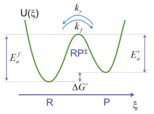
Our goal is to describe the rates of crossing the transition state for the forward and reverse reactions. At thermal equilibrium, the rate constants for the forward and reverse reaction, \( k_f \) and \( k_r \), are related to the equilibrium constant and the activation barriers as
\[K_{e q}=\frac{[P]}{[R]}=\frac{P_{P, e q}}{P_{R, e q}}=\frac{k_{f}}{k_{r}}=\exp \left(-\frac{\left(E_{a}^{f}-E_{a}^{r}\right)}{k_{B} T}\right) \nonumber \]
\(E^f_a\), \(E^r_a\) are the activation free energies for the forward and reverse reactions, which are related to the reaction free energy through \(E^f_a - E^r_a = \Delta G^0_{rxn}\). Pi refers to the population or probability of occupying the reactant or product state.
The primary assumptions of TST is that the transition state is well represented by an activated complex \(RP^‡\) that acts as an intermediate for the reaction from R to P, that all species are in thermal equilibrium, and that the flux across the barrier is proportional to the population of the activated complex.
\[R \rightleftharpoons RP^‡ \rightleftharpoons P \nonumber \]
Then, the steady state population of the activated complex can be determined by an equilibrium constant that we can express in terms of the molecular partition functions.
Let’s focus on the rate of the forward reaction considering only the equilibrium
\[R \rightleftharpoons RP^‡ \nonumber \]
We relate the population of reactants within the reactant well to the population of the activated complex through an equilibrium constant
\[K^‡_{eq} = \dfrac{[RP^‡]}{[R]} \nonumber \]
which we will evaluate using partition functions for the reactant and activated complex
\[ K^‡_{eq} =\dfrac{q^‡/V}{q_R/V}e^{-E^f_a/k_BT} \nonumber \]
Then we write the forward flux in eq. (23.1) proportional to the population of activated complex
\[\begin{aligned}\langle J^‡\rangle &= v[RP^‡]\\ &= vK^‡_{eq}[R] \end{aligned} \nonumber \]
Here ν is the reaction frequency, which is the inverse of the transition state lifetime \(\tau_{mol}\). \( v^{-1}\) or \(\tau_{mol}\) reflects the time it takes to cross the transition state region.
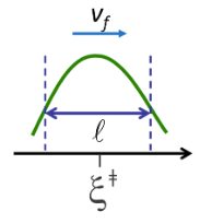
To evaluate ν, we will treat motion along the reaction coordinate ξ at the barrier as a translational degree of freedom. When the reactants gain enough energy (\(E^f_a\)), they will move with a constant forward velocity \(v_f\) through a transition state region that has a width \(\ell\). (The exact definition of \(\ell\) will not matter too much).
\[ \tau_{mol} = \dfrac{\ell}{v_f} \nonumber \]
Then we can write the average flux of population across the transition state in the forward direction
\[\begin{aligned} \langle J^‡\rangle &= K^‡_{eq} [R] \dfrac{v_f}{\ell}\\&= \dfrac{q^‡}{q_R}e^{-E^f_a/k_BT}[R] \frac{1}{\ell} \sqrt{\dfrac{k_BT}{2\pi m}} \end{aligned}\] \[\]
where \(v_f\) is obtained from a one-dimensional Maxwell–Boltzmann distribution.
For a multidimensional problem, we want to factor out the slow coordinate, i.e., reaction coordinate (ξ) from partition function.
\[ q^‡ = q_ξ q^{'‡} \nonumber \]
\(q^{'‡}\) contains all degrees of freedom except the reaction coordinate. Next, we calculate \(q_ξ\) by treating it as translational motion:
\[ q_ξ (trans) = \displaystyle\int\limits_0^{\ell} dξe^{-E_{trans}/k_BT} = \sqrt{\dfrac{2\pi m k_B T}{h^2}\ell} \]
Substituting (23.1.2) into (23.1.1):
\[\left\langle J_{f}^{‡}\right\rangle=\frac{k_{B} T}{h} \frac{q^{\prime ‡}}{q_{R}} e^{-E_{a}^{f} / k_{B} T}[R] \nonumber \]
We recognize that the factor \(v = k_BT/h\) is a frequency whose inverse gives an absolute lower bound on the crossing time of \(~10^{-13} \) seconds. If we use the speed of sound in condensed matter this time is what is needed to propagate 1–5 Å. Then we can write
\[\left\langle J_{f}^{‡}\right\rangle= k_f[R] \nonumber \]
where the forward rate constant is
\[k_f = Ae^{-E^f_a/k_BT} \]
and the pre-exponential factor is
\[ A = v\dfrac{q^{'‡}}{q_R} \nonumber \]
A determines the time that it takes to cross the transition state in the absence of barriers (Ea → 0). kf is also referred to as kTST.
To make a thermodynamic connection, we can express eq. (4) in the Eyring form
\[k_{f}=v e^{\Delta S^{‡} / k_{B}} e^{-\Delta E_{f}^{‡} / k_{B} T} \nonumber \]
where the transition state entropy is
\[ \Delta S^‡ = k\ln{\dfrac{q^{'‡}}{q_R}} \nonumber \]
\( \Delta S^‡\) represents a count (actually ratio) of the reduction of accessible microstates in making the transition from the reactant well to the transition state. For biophysical phenomena, the entropic factors are important, if not dominant!
Also note implicit in TST is a dynamical picture in which every trajectory that arrives with forward velocity at the TST results in a crossing. It therefore gives an upper bound on the true rate, which may include failed attempts to cross. This is often accounted for by adding a transmission coefficient κ < 1 to kTST: kf=κkTST. Kramers' theory provides a physical basis for understanding κ.