
17.3: Brownian Ratchet
- Page ID
- 294348

\( \newcommand{\vecs}[1]{\overset { \scriptstyle \rightharpoonup} {\mathbf{#1}} } \)
\( \newcommand{\vecd}[1]{\overset{-\!-\!\rightharpoonup}{\vphantom{a}\smash {#1}}} \)
\( \newcommand{\id}{\mathrm{id}}\) \( \newcommand{\Span}{\mathrm{span}}\)
( \newcommand{\kernel}{\mathrm{null}\,}\) \( \newcommand{\range}{\mathrm{range}\,}\)
\( \newcommand{\RealPart}{\mathrm{Re}}\) \( \newcommand{\ImaginaryPart}{\mathrm{Im}}\)
\( \newcommand{\Argument}{\mathrm{Arg}}\) \( \newcommand{\norm}[1]{\| #1 \|}\)
\( \newcommand{\inner}[2]{\langle #1, #2 \rangle}\)
\( \newcommand{\Span}{\mathrm{span}}\)
\( \newcommand{\id}{\mathrm{id}}\)
\( \newcommand{\Span}{\mathrm{span}}\)
\( \newcommand{\kernel}{\mathrm{null}\,}\)
\( \newcommand{\range}{\mathrm{range}\,}\)
\( \newcommand{\RealPart}{\mathrm{Re}}\)
\( \newcommand{\ImaginaryPart}{\mathrm{Im}}\)
\( \newcommand{\Argument}{\mathrm{Arg}}\)
\( \newcommand{\norm}[1]{\| #1 \|}\)
\( \newcommand{\inner}[2]{\langle #1, #2 \rangle}\)
\( \newcommand{\Span}{\mathrm{span}}\) \( \newcommand{\AA}{\unicode[.8,0]{x212B}}\)
\( \newcommand{\vectorA}[1]{\vec{#1}} % arrow\)
\( \newcommand{\vectorAt}[1]{\vec{\text{#1}}} % arrow\)
\( \newcommand{\vectorB}[1]{\overset { \scriptstyle \rightharpoonup} {\mathbf{#1}} } \)
\( \newcommand{\vectorC}[1]{\textbf{#1}} \)
\( \newcommand{\vectorD}[1]{\overrightarrow{#1}} \)
\( \newcommand{\vectorDt}[1]{\overrightarrow{\text{#1}}} \)
\( \newcommand{\vectE}[1]{\overset{-\!-\!\rightharpoonup}{\vphantom{a}\smash{\mathbf {#1}}}} \)
\( \newcommand{\vecs}[1]{\overset { \scriptstyle \rightharpoonup} {\mathbf{#1}} } \)
\( \newcommand{\vecd}[1]{\overset{-\!-\!\rightharpoonup}{\vphantom{a}\smash {#1}}} \)
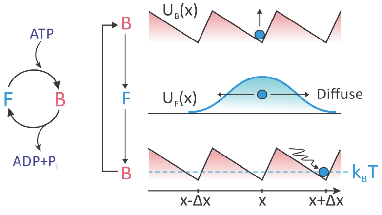
\(\newcommand{\avec}{\mathbf a}\) \(\newcommand{\bvec}{\mathbf b}\) \(\newcommand{\cvec}{\mathbf c}\) \(\newcommand{\dvec}{\mathbf d}\) \(\newcommand{\dtil}{\widetilde{\mathbf d}}\) \(\newcommand{\evec}{\mathbf e}\) \(\newcommand{\fvec}{\mathbf f}\) \(\newcommand{\nvec}{\mathbf n}\) \(\newcommand{\pvec}{\mathbf p}\) \(\newcommand{\qvec}{\mathbf q}\) \(\newcommand{\svec}{\mathbf s}\) \(\newcommand{\tvec}{\mathbf t}\) \(\newcommand{\uvec}{\mathbf u}\) \(\newcommand{\vvec}{\mathbf v}\) \(\newcommand{\wvec}{\mathbf w}\) \(\newcommand{\xvec}{\mathbf x}\) \(\newcommand{\yvec}{\mathbf y}\) \(\newcommand{\zvec}{\mathbf z}\) \(\newcommand{\rvec}{\mathbf r}\) \(\newcommand{\mvec}{\mathbf m}\) \(\newcommand{\zerovec}{\mathbf 0}\) \(\newcommand{\onevec}{\mathbf 1}\) \(\newcommand{\real}{\mathbb R}\) \(\newcommand{\twovec}[2]{\left[\begin{array}{r}#1 \\ #2 \end{array}\right]}\) \(\newcommand{\ctwovec}[2]{\left[\begin{array}{c}#1 \\ #2 \end{array}\right]}\) \(\newcommand{\threevec}[3]{\left[\begin{array}{r}#1 \\ #2 \\ #3 \end{array}\right]}\) \(\newcommand{\cthreevec}[3]{\left[\begin{array}{c}#1 \\ #2 \\ #3 \end{array}\right]}\) \(\newcommand{\fourvec}[4]{\left[\begin{array}{r}#1 \\ #2 \\ #3 \\ #4 \end{array}\right]}\) \(\newcommand{\cfourvec}[4]{\left[\begin{array}{c}#1 \\ #2 \\ #3 \\ #4 \end{array}\right]}\) \(\newcommand{\fivevec}[5]{\left[\begin{array}{r}#1 \\ #2 \\ #3 \\ #4 \\ #5 \\ \end{array}\right]}\) \(\newcommand{\cfivevec}[5]{\left[\begin{array}{c}#1 \\ #2 \\ #3 \\ #4 \\ #5 \\ \end{array}\right]}\) \(\newcommand{\mattwo}[4]{\left[\begin{array}{rr}#1 \amp #2 \\ #3 \amp #4 \\ \end{array}\right]}\) \(\newcommand{\laspan}[1]{\text{Span}\{#1\}}\) \(\newcommand{\bcal}{\cal B}\) \(\newcommand{\ccal}{\cal C}\) \(\newcommand{\scal}{\cal S}\) \(\newcommand{\wcal}{\cal W}\) \(\newcommand{\ecal}{\cal E}\) \(\newcommand{\coords}[2]{\left\{#1\right\}_{#2}}\) \(\newcommand{\gray}[1]{\color{gray}{#1}}\) \(\newcommand{\lgray}[1]{\color{lightgray}{#1}}\) \(\newcommand{\rank}{\operatorname{rank}}\) \(\newcommand{\row}{\text{Row}}\) \(\newcommand{\col}{\text{Col}}\) \(\renewcommand{\row}{\text{Row}}\) \(\newcommand{\nul}{\text{Nul}}\) \(\newcommand{\var}{\text{Var}}\) \(\newcommand{\corr}{\text{corr}}\) \(\newcommand{\len}[1]{\left|#1\right|}\) \(\newcommand{\bbar}{\overline{\bvec}}\) \(\newcommand{\bhat}{\widehat{\bvec}}\) \(\newcommand{\bperp}{\bvec^\perp}\) \(\newcommand{\xhat}{\widehat{\xvec}}\) \(\newcommand{\vhat}{\widehat{\vvec}}\) \(\newcommand{\uhat}{\widehat{\uvec}}\) \(\newcommand{\what}{\widehat{\wvec}}\) \(\newcommand{\Sighat}{\widehat{\Sigma}}\) \(\newcommand{\lt}{<}\) \(\newcommand{\gt}{>}\) \(\newcommand{\amp}{&}\) \(\definecolor{fillinmathshade}{gray}{0.9}\)The Brownian ratchet refers to a class of models for directed transport using Brownian motion that is rectified through the input of energy. For a diffusing particle, the energy is used to switch between two states that differ in their diffusive transport processes. This behavior results in biased diffusion. It is broadly applied for processive molecular motors stepping between discrete states, and it therefore particularly useful for understanding translational and rotational motor proteins.
One common observation we find is that directed motion requires the object to switch between two states that are coupled to its motion, and for which the exchange is driven by input energy. Switching between states results in biased diffusion. The interpretation of real systems within the context of this model can vary. Some people consider this cycle as deterministic, whereas others consider it quite random and noisy, however, in either case, Brownian motion is exploited to an advantage in moving the particle.
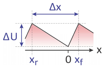
We will consider an example relevant to the ATP-fueled stepping of cytoskeletal motors along a filament. The motor cycles between two states: (1) a bound state (B), for which the protein binds to a particular site on the filament upon itself binding ATP, and (2) a free state (F) for which the protein freely diffuses along the filament upon ATP hydrolysis and release of ADP + Pi. The bound state is described by a periodic, spatially asymmetric energy profile \(U_B(x)\), for which the protein localizes to a particular energy minimum along the filament. Key characteristics of this potential are a series of sites separated by a barrier \(ΔU > k_BT\), and an asymmetry in each well that biases the system toward a local minimum in the direction of travel. In the free state, there are no barriers to motion and the protein diffuses freely. When the free protein binds another ATP, it returns to \(U_B(x)\) and relaxes to the nearest energy minimum.
Let’s investigate the factors governing the motion of the particle in this Brownian ratchet, using the perspective of a biased random walk. The important parameters for our model are:
- The distance between adjacent binding sites is \(Δx\).
- The position of the forward barrier relative to the binding site is \(x_f\). A barrier for reverse diffusion is at \(–x_r\), so that
\[x_f+x_r = \Delta x\]
The asymmetry of \(U_B\) is described by
\[ \alpha =(x_f-x_r)/\Delta x \]
- The average time that a ratchet stays free or bound are \(\tau_F\) and \(\tau_B\). Therefore, the average time per bind/release cycle is
\[ \Delta t = \tau_F+\tau_B \nonumber \]
- We define a diffusion length \(\ell \) which is dependent on the time that the protein is free
\[ \ell_0(\tau_F)=\sqrt{4D\tau_F} \nonumber \]
Conditions For Efficient Transport
Let’s consider the conditions to maximize the velocity of the Brownian ratchet.
- While in \(F\): the optimal period to be diffusing freely is governed by two opposing concerns. We want the particle to be free long enough to diffuse past the forward barrier, but not so long that it diffused past the reverse barrier. Thus we would like the diffusion length to lie between the distances to these barriers:
\[ \ell_0=\sqrt{4D\tau_F} \nonumber \]
\[ x_r > l_0 > x_F \nonumber \]
Using the average value as a target:
\[ \begin{aligned} \ell_0 &\approx \dfrac{x_r+x_F}{2}= \dfrac{\Delta x}{2} \\ \tau_F &\approx \dfrac{\Delta x^2}{16D} \end{aligned} \]
2. While in B: After the binding ATP, we would like the particle to stay with ATP bound long enough to relax to the minimum of the asymmetric energy landscape. Competing with this consideration, we do not want it to stay bound any longer than necessary if speed is the issue.
We can calculate the time needed to relax from the barrier at xr forward to the potential minimum, if we know the drift velocity vd of this particle under the influence of the potential.
\[\tau_B \approx x_r/ \nu_d \nonumber \]
The drift velocity is related to the force on the particle through the friction coefficient, \(\nu_d = f/\zeta \), and we can obtain the magnitude of the force from the slope of the potential:
\[ |f| = \dfrac{\Delta U}{x_r} \nonumber \]
So the drift velocity is \(\nu_d = \dfrac{fD}{k_BT}= \dfrac{\Delta UD}{x_rk_BT} \) and the optimal bound time is
\[\tau_B \approx \dfrac{x_r^2k_BT}{\Delta UD} \nonumber \]
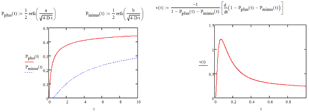
Now let’s look at this a bit more carefully. We can now calculate the probability of diffusing forward over the barrier during the free interval by integrating over the fraction of the population that has diffused beyond xf during τF. Using the diffusive probability distribution with x0→0,
\[ \begin{aligned} P_+ &= \dfrac{1}{\sqrt{4\pi D\tau_F}} \int_{x_f}^{\infty} e^{-x^2/4D\tau_F} dx \\ &=\dfrac{1}{2} erfc\left( \dfrac{x_f}{\ell_0} \right) \end{aligned}\]
Similarly, the probability for diffusing backward over the barrier at x = ‒xr is
\[ P_- = \dfrac{1}{2} erfc \left( \dfrac{x_r}{\ell_0} \right) \nonumber \]
Now we can determine the average velocity of the protein by calculating the average displacement in a given time step. The average displacement is the difference in probability for taking a forward versus a reverse step, times the step size. This displacement occurs during the time interval Δt. Therefore,
\[ \begin{aligned} \nu &= \dfrac{\Delta P \Delta x}{\Delta t}\\ &=\dfrac{(P_+-P_-)\Delta x}{(\tau_B + \tau_F)} \\ &=\dfrac{\Delta x}{2\Delta t} \left[ erf\left( \dfrac{x_r}{\ell_0 (\tau_F)}\right) - erf \left( \dfrac{x_f}{\ell_0 (\tau_F)} \right) \end{aligned} \]
It is clear from this expression that the velocity is zero when the asymmetry of the potential is zero. For asymmetric potentials, P+ and P‒ are dependent on τF, with one rising in time faster than the other. As a result, the velocity, which depends on the difference of these reaches a maximum in the vicinity of \(\tau_F=x^2_f/D \).
So how does the ATP hydrolysis influence the free energy gradient? Here free energy gradient is
\[ \dfrac{\Delta G_{Hyd.}}{\Delta x} \nonumber \]

\(k_+ = A_+e^{-(\Delta G_{barrier}-\Delta G_{hydrolysis})/kT} \)
\(k_- = A_-e^{-(\Delta G_{barrier})/kT} \)
\( \nu = (k_+-k_-) \Delta x \)
___________________________________________
K. Dill and S. Bromberg, Molecular Driving Forces: Statistical Thermodynamics in Biology, Chemistry, Physics, and Nanoscience. (Taylor & Francis Group, New York, 2010); R. Phillips, J. Kondev, J. Theriot and H. Garcia, Physical Biology of the Cell, 2nd ed. (Taylor & Francis Group, New York, 2012).