
13.1: Langevin Equation
- Page ID
- 294330

\( \newcommand{\vecs}[1]{\overset { \scriptstyle \rightharpoonup} {\mathbf{#1}} } \)
\( \newcommand{\vecd}[1]{\overset{-\!-\!\rightharpoonup}{\vphantom{a}\smash {#1}}} \)
\( \newcommand{\id}{\mathrm{id}}\) \( \newcommand{\Span}{\mathrm{span}}\)
( \newcommand{\kernel}{\mathrm{null}\,}\) \( \newcommand{\range}{\mathrm{range}\,}\)
\( \newcommand{\RealPart}{\mathrm{Re}}\) \( \newcommand{\ImaginaryPart}{\mathrm{Im}}\)
\( \newcommand{\Argument}{\mathrm{Arg}}\) \( \newcommand{\norm}[1]{\| #1 \|}\)
\( \newcommand{\inner}[2]{\langle #1, #2 \rangle}\)
\( \newcommand{\Span}{\mathrm{span}}\)
\( \newcommand{\id}{\mathrm{id}}\)
\( \newcommand{\Span}{\mathrm{span}}\)
\( \newcommand{\kernel}{\mathrm{null}\,}\)
\( \newcommand{\range}{\mathrm{range}\,}\)
\( \newcommand{\RealPart}{\mathrm{Re}}\)
\( \newcommand{\ImaginaryPart}{\mathrm{Im}}\)
\( \newcommand{\Argument}{\mathrm{Arg}}\)
\( \newcommand{\norm}[1]{\| #1 \|}\)
\( \newcommand{\inner}[2]{\langle #1, #2 \rangle}\)
\( \newcommand{\Span}{\mathrm{span}}\) \( \newcommand{\AA}{\unicode[.8,0]{x212B}}\)
\( \newcommand{\vectorA}[1]{\vec{#1}} % arrow\)
\( \newcommand{\vectorAt}[1]{\vec{\text{#1}}} % arrow\)
\( \newcommand{\vectorB}[1]{\overset { \scriptstyle \rightharpoonup} {\mathbf{#1}} } \)
\( \newcommand{\vectorC}[1]{\textbf{#1}} \)
\( \newcommand{\vectorD}[1]{\overrightarrow{#1}} \)
\( \newcommand{\vectorDt}[1]{\overrightarrow{\text{#1}}} \)
\( \newcommand{\vectE}[1]{\overset{-\!-\!\rightharpoonup}{\vphantom{a}\smash{\mathbf {#1}}}} \)
\( \newcommand{\vecs}[1]{\overset { \scriptstyle \rightharpoonup} {\mathbf{#1}} } \)
\( \newcommand{\vecd}[1]{\overset{-\!-\!\rightharpoonup}{\vphantom{a}\smash {#1}}} \)
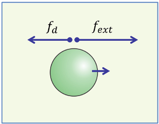
\(\newcommand{\avec}{\mathbf a}\) \(\newcommand{\bvec}{\mathbf b}\) \(\newcommand{\cvec}{\mathbf c}\) \(\newcommand{\dvec}{\mathbf d}\) \(\newcommand{\dtil}{\widetilde{\mathbf d}}\) \(\newcommand{\evec}{\mathbf e}\) \(\newcommand{\fvec}{\mathbf f}\) \(\newcommand{\nvec}{\mathbf n}\) \(\newcommand{\pvec}{\mathbf p}\) \(\newcommand{\qvec}{\mathbf q}\) \(\newcommand{\svec}{\mathbf s}\) \(\newcommand{\tvec}{\mathbf t}\) \(\newcommand{\uvec}{\mathbf u}\) \(\newcommand{\vvec}{\mathbf v}\) \(\newcommand{\wvec}{\mathbf w}\) \(\newcommand{\xvec}{\mathbf x}\) \(\newcommand{\yvec}{\mathbf y}\) \(\newcommand{\zvec}{\mathbf z}\) \(\newcommand{\rvec}{\mathbf r}\) \(\newcommand{\mvec}{\mathbf m}\) \(\newcommand{\zerovec}{\mathbf 0}\) \(\newcommand{\onevec}{\mathbf 1}\) \(\newcommand{\real}{\mathbb R}\) \(\newcommand{\twovec}[2]{\left[\begin{array}{r}#1 \\ #2 \end{array}\right]}\) \(\newcommand{\ctwovec}[2]{\left[\begin{array}{c}#1 \\ #2 \end{array}\right]}\) \(\newcommand{\threevec}[3]{\left[\begin{array}{r}#1 \\ #2 \\ #3 \end{array}\right]}\) \(\newcommand{\cthreevec}[3]{\left[\begin{array}{c}#1 \\ #2 \\ #3 \end{array}\right]}\) \(\newcommand{\fourvec}[4]{\left[\begin{array}{r}#1 \\ #2 \\ #3 \\ #4 \end{array}\right]}\) \(\newcommand{\cfourvec}[4]{\left[\begin{array}{c}#1 \\ #2 \\ #3 \\ #4 \end{array}\right]}\) \(\newcommand{\fivevec}[5]{\left[\begin{array}{r}#1 \\ #2 \\ #3 \\ #4 \\ #5 \\ \end{array}\right]}\) \(\newcommand{\cfivevec}[5]{\left[\begin{array}{c}#1 \\ #2 \\ #3 \\ #4 \\ #5 \\ \end{array}\right]}\) \(\newcommand{\mattwo}[4]{\left[\begin{array}{rr}#1 \amp #2 \\ #3 \amp #4 \\ \end{array}\right]}\) \(\newcommand{\laspan}[1]{\text{Span}\{#1\}}\) \(\newcommand{\bcal}{\cal B}\) \(\newcommand{\ccal}{\cal C}\) \(\newcommand{\scal}{\cal S}\) \(\newcommand{\wcal}{\cal W}\) \(\newcommand{\ecal}{\cal E}\) \(\newcommand{\coords}[2]{\left\{#1\right\}_{#2}}\) \(\newcommand{\gray}[1]{\color{gray}{#1}}\) \(\newcommand{\lgray}[1]{\color{lightgray}{#1}}\) \(\newcommand{\rank}{\operatorname{rank}}\) \(\newcommand{\row}{\text{Row}}\) \(\newcommand{\col}{\text{Col}}\) \(\renewcommand{\row}{\text{Row}}\) \(\newcommand{\nul}{\text{Nul}}\) \(\newcommand{\var}{\text{Var}}\) \(\newcommand{\corr}{\text{corr}}\) \(\newcommand{\len}[1]{\left|#1\right|}\) \(\newcommand{\bbar}{\overline{\bvec}}\) \(\newcommand{\bhat}{\widehat{\bvec}}\) \(\newcommand{\bperp}{\bvec^\perp}\) \(\newcommand{\xhat}{\widehat{\xvec}}\) \(\newcommand{\vhat}{\widehat{\vvec}}\) \(\newcommand{\uhat}{\widehat{\uvec}}\) \(\newcommand{\what}{\widehat{\wvec}}\) \(\newcommand{\Sighat}{\widehat{\Sigma}}\) \(\newcommand{\lt}{<}\) \(\newcommand{\gt}{>}\) \(\newcommand{\amp}{&}\) \(\definecolor{fillinmathshade}{gray}{0.9}\)Consider the forces acting on a particle as we pull it through a fluid. We pull the particle with an external force \(f_{ext}\), which is opposed by a drag force from the fluid, \(f_d\). The drag or damping acts as resistance to motion of the particle, which results from trying to move the fluid out of the way.
\[f_d = -\zeta v \qquad \qquad \quad \zeta \mathrm{(kg/s)} \]
A drag force requires movement, so it is proportional to the velocity of the particle \(v=dx/dt=x\) and the friction coefficient \(\zeta\) is the proportionality constant that describes the magnitude of the damping. Newton’s second law relates the acceleration of this particle is to the sum of these forces:
\[ ma = f_d+f_{ext} \nonumber \]
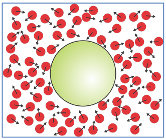
Now microscopically, we also recognize that there are time-dependent random forces that the molecules of the fluid exert on a molecule (\(f_r\)). So that the specific molecular details of solute–solvent collisions can be averaged over, it is useful to think about a nanoscale solute in water (e.g., biological macromolecules) with dimensions large enough that its position is simultaneously influenced by many solvent molecules, but is also light enough that the constant interactions with the solvent leave an unbalanced force acting on the solute at any moment in time:
\[\overline{f}_r(t)=-\sum_i \overline{f}_i(t) \nonumber\]
Then Newton’s second law is
\[ ma = f_d + f_{ext} +f_r(t) \nonumber \]
The drag force is present regardless of whether an external force is present, so in the absence of external forces (\(f_{ext}=0\)) the equation of motion governing the spontaneous fluctuations of this solute is determined from the forces due to drag and the random fluctuations:
\[ma = f_d + f_r(t) \label{13.1.1}\]
\[m\ddot{x} + \zeta \dot{x} - f_r(t) = 0 \label{13.1.2}\]
This equation of motion is the Langevin equation. An equation of motion such as this that includes a time-dependent random force is known as “stochastic”.
Inserting a random process into a deterministic equation means that we need to use a statistical approach to solve this equation. We will be looking to describe the average and root-mean-squared position of the particle. First, what can we say about the random force? Although there may be momentary imbalances, on average the perturbations from the solvent on a larger particle will average to zero at equilibrium:
\[ \langle f_r(t) \rangle = 0 \]
Equation \ref{13.1.1} seems to imply that the drag force and the random force are independent, but in fact they originate in the same molecular forces. If the molecule of interest is a protein that experiences the fluctuations of many rapidly moving solvent molecules, then the averaged forces due to random fluctuations and the drag forces are related. The fluctuation–dissipation theorem is the general relationship that relates the friction to the correlation function for the random force. In the Markovian limit this is
\[ \langle f_r(t) f_r(t') \rangle = 2\zeta k_BT \delta (t-t')\]
or \[ \zeta = \dfrac{\langle f_r^2 \rangle }{2k_BT} \nonumber \]
Markovian indicates that no correlation exists between the random force for |t‒t′| > 0. More generally, we can recover the friction coefficient from the integral over the correlation function for the random force
\[ \zeta = \dfrac{1}{2k_BT} \int^{+\infty}_{-\infty} dt \langle f_R(0)f_R(t) \rangle \nonumber \]
To describe the time evolution of the position of our protein molecule, we would like to obtain an expression for mean-square displacement ⟨x2(t)⟩. The position of the molecule can be described by integrating over its time-dependent velocity: \(x(t)=\int^t_0 dt' \dot{x}(t')\), so we can express the mean-square displacement in terms of the velocity autocorrelation function
\[\langle x^2(t) \rangle = \int^t_0 dt' \int^t_0 dt'' \langle \dot{x}(t') \dot{x}(t'') \rangle \]
Our approach to obtaining ⟨x2(t)⟩ starts by multiplying eq. (13.1.2) by x and then ensemble averaging.
\[ m \langle x \dfrac{d}{dt} \dot{x} \rangle + \zeta \langle x \dot{x} \rangle - \langle xf_r(t) \rangle =0 \]
From eq. (13.1.3), the last term is zero, and from the chain rule we know
\[ \dfrac{d}{dt} (x\dot{x}) = x\dfrac{d}{dt} \dot{x} + \dfrac{dx}{dt}\dot{x} \]
Therefore, we can write eq. (13.1.6) as
\[ m \left( \dfrac{d}{dt} \langle x\dot{x} \rangle - \langle \dot{x} \dot{x} \rangle \right) + \zeta \langle x \dot{x} \rangle = 0 \]
Further, the equipartition theorem states that for each translational degree of freedom the kinetic energy is partitioned as
\[ \dfrac{1}{2} m \langle \dot{x}^2 \rangle = \dfrac{k_BT}{2} \]
So, \[m \dfrac{d}{dt} \langle x\dot{x} \rangle + \zeta \langle x \dot{x} \rangle = k_BT \]
Here we are describing motion in 1D, but when fluctuations and displacement are included for 3D motion, then we switch x → r and kBT→3kBT. Integrating eq. (13.1.10) twice with respect to time, and using the initial condition x(0) = 0, we obtain
\[ \langle x^2 \rangle = \dfrac{2k_BT}{\zeta } \left\{ t +\dfrac{m}{\zeta } \left[ \exp \left( -\dfrac{\zeta }{m}t \right) -1 \right] \right\} \]
in 3D:
\[\langle r^2 \rangle = \dfrac{6k_BT}{\zeta } \left\{ t +\dfrac{m}{\zeta } \left[ \exp \left( -\dfrac{\zeta }{m}t \right) -1 \right] \right\} \nonumber \]
To investigate eq. (13.1.11), let’s consider two limiting cases. We see that m/ζhas units of time, and so we define the relaxation time
\[ \tau_C = m/ \zeta \]
and investigate time scale short and long compared to τC:
1) For \(t \ll \tau_C \), we can expand the exponential in eq. (11) and retain the first three terms, which leads to
\[ \langle x^2 \rangle \approx \dfrac{k_BT}{m}t^2 = \langle v^2 \rangle t^2 \qquad \qquad \quad \text{(short time: inertial)}\]
2) For \(t \gg \tau_C\), eq. (11) is dominated by the leading term:
\[ \langle x^2 \rangle = \dfrac{2k_BT}{\zeta} t \qquad \qquad \quad \text{(long time: diffusive)} \]
In the diffusive limit the behavior of the molecule is governed entirely by the fluid, and its mass does not matter. The diffusive limit in a stochastic equation of motion is equivalent to setting m→0.
We see that τC is a time-scale separating motion in the inertial and diffusive limits. It is a correlation time for the randomization of the velocity of the particle due to the random fluctuations of the environment.
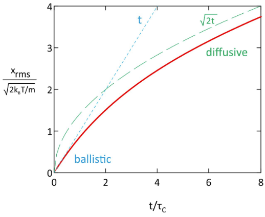
For very little friction or short time, the particle moves with traditional deterministic motion xrms= vrms t, where root-mean-square displacement xrms = ⟨x2⟩1/2 and vrms comes from the average translational kinetic energy of the particle. For high-friction or long times, we see diffusive behavior with xrms~t1/2. Furthermore, by comparing eq. (13.1.14) to our earlier continuum result, ⟨x2⟩ = 2Dt, we see that the diffusion constant can be related to the friction coefficient by
\[ D= \dfrac{k_BT}{\zeta} \quad \text{(in 1D)} \]
This is the Einstein formula. For 3D problems, we replace kBT with 3kBT in the expressions above and find \( D_{3D}=3k_BT /\zeta\).
\[ \tau_C = \dfrac{m}{\zeta} = \dfrac{mD}{k_BT} \quad \text{(in 1D)} \nonumber \]
How long does it take to approach the diffusive regime? Very fast. Consider a 100 kDa protein with R = 3 nm in water at T = 300 K, we find a characteristic correlation time for randomizing velocities of \(\tau_C=3\mathrm{x}10^{-12}\) s, which corresponds to a distance of about 10–2 nm before the onset of diffusive behavior.
We can find other relationships. Noting the relationship of ⟨x2⟩ to the velocity autocorrelation function in eq. (13.1.5), we find that the particle velocity is described by
\[ \langle v_x(0)v_x(t) \rangle = \langle v_x^2\rangle e^{-\zeta t /m}= \langle v^2_x \rangle e^{-t/\tau_C} \qquad \qquad \qquad v_x = \dot{x} \nonumber \]
which can be integrated over time to obtain the diffusion constant.
\[ \int^{\infty}_0 \langle v_x(0)v_x(t) \rangle dt = \dfrac{k_BT}{\zeta} = D \]
This expression is the Green–Kubo relationship. This is a practical way of analyzing molecular trajectories in simulations or using particle-tracking experiments to quantify diffusion constants or friction coefficients.