6.1: Electrostatics

Electrical Properties of Water and Aqueous Solutions

We want to understand the energy and electrical properties and transport of ions and charged molecules in water. These are strong forces. Consider an example of \(\ce{NaCl}\) dissociation in gas phase dissociation energy \(\Delta H_{\text{ionization}} \approx 270\ kJ/mol\):

\[K_{\text {ioniztion }}(\text { gas })=\dfrac{\left[\mathrm{Na}^{+}\right]\left[\mathrm{Cl}^{-}\right]}{[\mathrm{NaCl}]} \approx 10^{-89}
\nonumber\]

In solution, this process [\(\ce{NaCl} (aq) \to \text{Na}^+ (aq) + \text{Cl}^- (aq)\)] occurs spontaneously; the solubility product for \(\ce{NaCl}\) is \(K_{\text{sp}} = [\text{Na}^+ (aq)][\text{Cl}^- (aq)] / [\ce{NaCl} (aq)] = 37\). Similarly, water molecules are covalently bonded hydrogen and oxygen atoms, but we know that the internal forces in water can autoionize a water molecule:

\[K_{\text {ionization }}(\text { gas })=\left[\mathrm{H}^{+}\right]\left[\mathrm{OH}^{-}\right] \approx 10^{-75} \text { and } K_{W}\left(\mathrm{H}_{2} \mathrm{O}\right) = \left[\mathrm{H}^{+}\right] \left [\mathrm{OH}^{-} \right]=10^{-14} \nonumber\]

These tremendous differences originate in the huge collective electrostatic forces that are present in water. “Polar solvation” refers to the manner in which water dipoles stabilize charges.

These dipoles are simplifications of the rearrangements of water’s structure to accommodate and lower the energy of the ion. It is important to remember that water is a polarizable medium in which hydrogen bonding dramatically modifies the electrostatic properties.

Electrostatics

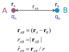
Let’s review a number of results from classical electrostatics. The interactions between charged objects can be formulated using force, the electric field, or the electrostatic potential. The potential is our primary consideration when discussing free energies in thermodynamics and the Hamiltonian in statistical mechanics. Let’s describe these, consider the interaction between two ions \(A\) and \(B\), separated by a distance \(r_{AB}\), with charges \(q_A\) and \(q_B\).

Force and Work

Coulomb’s Law gives the force that \(B\) exerts on \(A\).

\[\boldsymbol{f}_{A B}=-\dfrac{1}{4 \pi \varepsilon} \dfrac{q_{A} q_{B}}{r_{A B}^{2}} \hat{r}_{A B}\nonumber\]

\(\hat{r}_{AB}\) is a unit vector pointing from \(\mathbf{r}_B\) to \(\mathbf{r}_A\). A useful identity to remember for calculations is

\[\dfrac{e^{2}}{4 \pi \varepsilon_{0}}=230 p N /n m^{2}\nonumber\]

For thermodynamic purposes it is helpful to calculate the reversible work for a process. Electrical work comes from moving charges against a force

\[d w=-\boldsymbol{f} \cdot d \mathbf{r} \nonumber\]

As long as q and ε are independent of r, and the process is reversible, then work only depends on r, and is independent of path. To move particle B from point 1 at a separation r₀ to point 2 at a separation r requires the following work\[
w_{1 \rightarrow 2}=\frac{1}{4 \pi \varepsilon} q_{A} q_{B}\left(\frac{1}{r_{2}}-\frac{1}{r_{1}}\right)
\]

and if the path returns to the initial position, \(w_{rev} = 0\).

Field, E

The electric field is a vector quantity that describes the action of charges at a point in space. The field from charged particle \(B\) at point \(A\) is

\[\mathbf{E}_{A B}\left(\mathbf{r}_{A}\right)=-\dfrac{1}{4 \pi \varepsilon} \frac{q_{B}}{r_{A B}^{2}} \hat{r}_{A B} \nonumber\]

\(\mathbf{E}_{AB}\) is related to the force that particle \(B\) exerts on a charged test particle \(A\) with charge \(q_A\) through

\[\mathbf{f}_{A} = q_{A} \mathbf{E}_{A B}\left(\mathbf{r}_{A}\right)\nonumber\]

While the force at point a depends on the sign and magnitude of the test charge, the field does not. More generally, the field exerted by multiple charged particles at point \(\mathbf{r}_A\) is the vector sum of the field from multiple charges (\(i\)):

\[\mathbf{E}\left(\mathbf{r}_{A}\right)=\sum_{i} \mathbf{E}_{A i}\left(\mathbf{r}_{A}\right)=-\dfrac{1}{4 \pi \varepsilon} \sum_{i} \dfrac{q_{i}}{r_{A i}^{2}} \hat{r}_{A i}\nonumber\]

where \(r_{Ai} = \left |\mathbf{r}_A - \mathbf{r}_i \right|\) and the unit vector \(\hat{A}_{Ai} = (\mathbf{r}_A - \mathbf{r}_i)/r_{Ai}\). Alternatively for a continuum charge density \(\rho_q (\mathbf{r})\),

\[\mathbf{E}\left(\mathbf{r}_{A}\right)=-\dfrac{1}{4 \pi \varepsilon} \int \rho_{q}(\mathbf{r}) \dfrac{\left(\mathbf{r}_{A}-\mathbf{r}\right)}{\left|\mathbf{r}_{A}-\mathbf{r}\right|^{3}} d \mathbf{r}\nonumber\]

where the integral is over a volume.

Electrostatic Potential, \(\Phi\)

For thermodynamics and statistical mechanics, we wish to express electrical interactions in terms of an energy or electrostatic potential. While the force and field are vector quantities, the electrostatic potential \(\Phi\) is a scalar quantity which is related to the electric field through

\[\mathbf{E}=-\bar{\nabla} \Phi \nonumber\]

It has units of energy per unit charge. The electrostatic potential at point \(\mathbf{r}_A\), which results from a point charge at \(\mathbf{r}_B\), is

\[\Phi \left(r_{A}\right)=\dfrac{1}{4 \pi \varepsilon} \dfrac{q_{B}}{r_{A B}}\]

The electric potential is additive in the contribution from multiple charges:

\[
\Phi\left(r_{A}\right)=\dfrac{1}{4 \pi \varepsilon} \sum_{i} \dfrac{q_{i}}{r_{A i}} \quad \text { or } \quad \Phi\left(r_{A}\right)=\dfrac{1}{4 \pi \varepsilon} \int \dfrac{\rho_{q}(\mathbf{r})}{\left|\mathbf{r}_{A}-\mathbf{r}\right|} d \mathbf{r}
\nonumber\]

The electrostatic energy of a particle \(A\) as a result of the potential due to particle \(B\) is

\[
U_{A B}\left(r_{A}\right)=q_{A} \Phi\left(r_{A}\right)=\dfrac{1}{4 \pi \varepsilon} \dfrac{q_{A} q_{B}}{r_{A B}}\nonumber
\]

Note that \(U_{A B}=q_{A} \Phi\left(r_{A}\right)=q_{B} \Phi\left(r_{B}\right)=\tfrac{1}{2}\left(q_{A} \Phi\left(r_{A}\right)+q_{B} \Phi\left(r_{B}\right)\right)\), so we can generalize this to calculate the potential energy stored in a collection of multiple charges as

\[
\begin{aligned}
U &=\dfrac{1}{2} \sum_{i} q_{i} \Phi\left(r_{A i}\right) \\
&=\frac{1}{2} \int \Phi_{A}\left(\mathbf{r}_{A}\right) \rho_{q}\left(\mathbf{r}_{A}\right) d \mathbf{r}_{A}
\end{aligned} \nonumber
\]