2.3: Binary Fluid

Entropy of Mixing

The thermodynamics of the mixing process is important to phase equilibria, hydrophobicity, solubility, and related solvation problems. The process of mixing two pure substances \(A\) and \(B\) is shown below. We define the composition of the system through the number of \(A\) and \(B\) particles: \(N_A\) and \(N_B\) and the total number of particles \(N = N_A + N_B\), which also equals the number of cells. We begin with two containers of the homogeneous pure fluids and mix them together, keeping the total number of cells constant. In the case of the pure fluids before mixing, all cells of the container are initially filled, so there is only one accessible microstate, \(\Omega_{\text{pure}} = 1\), and

\[S_{\text{pure}} = k_B \ln 1 = 0\nonumber\]

When the two containers are mixed, the number of possible microstates are given by the binomial distribution: \(\Omega_{\text{mix}} = N!/N_A! N_B!\).

If these particles have no interactions, each microstate is equally probable, and similar to eq. (2.2.2) we obtain the entropy of the mixture as

\[S_{\text{mix}}=-N k_{B}\left(x_{A} \ln x_{A}+x_{B} \ln x_{B}\right) \label{eq2.3.1}\]

For the mixture, we define the mole fractions for the two components: \(x_A = N_A / N\) and \(x_B = N_B / N\). As before, since \(x_A\) and \(x_B < 1\), the entropy for the mixture is always positive. The entropy of mixing is then calculated from \(\Delta S_{\text{mix}} = S_{\text{mix}} - (S_{\text{pure A}} + S_{\text{pure B}})\). Since the entropy of the pure substances in this model is zero, \(\Delta S_{\text{mix}} = S_{\text{mix}}\). A plot of this function as a function of mole fractions illustrates that the maximum entropy mixture has \(x_A = x_B = 0.5\).

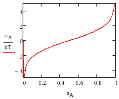
In the absence of interactions between particles, the free energy of mixing is purely entropic with \(\Delta F_{\text{mix}} = -T \Delta S_{\text{mix}}\). The chemical potential of \(A\) particles \(\mu_A\) describes the free energy needed to replace a particle \(B\) with an additional \(A\) particle, and is obtained from

\[\begin{array} {l} {\mu_i = \left (\dfrac{\partial F}{\partial N_i} \right )_{T, V, \{N_{j \ne i}\}}} \\ {\mu_A = -k_B T (\ln x_A - \ln x_B) = -\mu B} \end{array} \nonumber\]

This curve illustrates the increasing challenge of finding available space as the packing fraction increases.

Intermolecular Interaction

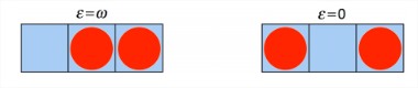
To look at real systems, we now add interactions between particles by assigning an interaction energy \(\omega\) between two cells which are in contact. The interaction energy can be positive (destabilizing) or negative (favorable).

With the addition of intermolecular interactions, each microstate will have a distinct energy, the canonical partition function can be obtained from eq. (2.1.1), and other thermodynamic properties follow.

In the case of a mixture, we assign separate interaction energies for each adjoining \(A-A\), \(B-B\), or \(A-B\) pair in a given microstate: \(\omega_{AA}, \omega_{BB}, \omega_{AB}\). How do we calculate the energy of a microstate? m is the total number of molecular contacts in the volume, and these can be divided into \(A-A\), \(B-B\), or \(A-B\) contacts:

\[m = m_{AA} + m_{BB} + m_{AB} \nonumber\]

While \(m\) is constant, the counts of specific contacts \(m_{ij}\) vary by microstate. Then the energy of the mixture for the single \(i^{th}\) microstate can be written as

\[E_{\text {mix}}=m_{A A} \omega_{A A}+m_{B B} \omega_{B B}+m_{A B} \omega_{A B} \label{eq2.3.2}\]

and the internal energy comes from an ensemble average of this quantity. An exact calculation of the internal energy from the partition function would require a sum over all possible configurations with their individual contact numbers. Instead, we can use a simpler, approximate approach which uses a strategy that starts by expressing each term in eq. (\(\ref{eq2.3.2}\)) in terms of \(m_{AB}\). We know:

\[\begin{array} {rcl} {m_{AA}} & = & {\text{(Total contacts for A) - (Contacts of A with B)}} \\ {} & = & {\dfrac{zN_A}{2} - \dfrac{m_{AB}}{2}} \end{array}\]

\[m_{B B}=\dfrac{z N_{B}}{2}-\dfrac{m_{A B}}{2}\]

Then we have

\[\begin{array} {rcl} {E_{\text{mix}}} & = & {\left (\dfrac{z\omega_{AA} N_A}{2} \right ) + \left (\dfrac{z\omega_{BB} N_B}{2} \right ) + m_{AB} \left (\omega_{AB} - \dfrac{\omega_{AA} + \omega_{BB}}{2} \right )} \\ {} & = & {U_{\text{pure A}} + U_{\text{pure B}} + m_{AB} \Delta \omega} \end{array} \label{eq2.3.5}\]

The last term in this expression is half the change of interaction energy to switch an \(A-A\) and a \(B-B\) contact to form two \(A-B\) contacts:

\[\Delta \omega = \left (\omega_{A B} - \dfrac{\omega_{A A} + \omega_{B B}}{2} \right)\]

We also recognize that the first two terms are just the energy of the two pure liquids before mixing. These are calculated by taking the number of cells in the pure liquid (\(N_i\)) times the number of contacts per cell (\(z\)) and then divide by two, so you do not double count the contacts.

\[U_{\text{pure, i}} = \dfrac{z \omega_{ii} N_{i}}{2}\]

With these expressions, eq. (\(\ref{eq2.3.5}\)) becomes

\[E_{\text{mix}} = U_{\text{pure A}} + U_{\text{pure B}} + m_{AB} \Delta \omega \nonumber\]

This equation describes the energy of a microstate in terms of the number of \(A-B\) contacts present \(m_{AB}\).

At this point, this is not particularly helpful because it is not practical to enumerate all of the possible microstates and their corresponding \(m_{AB}\). To simplify our calculation of \(U_{\text{mix}}\), we make a "mean field approximation," which replaces \(m_{AB}\) with its statistical average \(\langle m_{AB} \rangle\):

\[\begin{array} {rcl} {\langle m_{AB} \rangle} & = & {\text{(# of contact sites for A)} \times \text{(probability of contact site being B)}} \\ {} & = & {(N_A z) \left (\dfrac{N_B}{N}\right ) = zx_A x_B N} \end{array}\]

Then for the energy for the mixed state \(U_{\text{mix}} = \langle E_{\text{mix}} \rangle\), we obtain:

\[U_{\text{mix}} = U_{\text{pure A}} + U_{\text{pure B}} + x_A x_B Nk_B T \chi_{AB}\]

Here we have introduced the unitless exchange parameter,

\[\chi_{A B}=\dfrac{z}{k_{B} T} \left (\omega_{A B} - \dfrac{\omega_{A A}+\omega_{B B}}{2} \right ) = \dfrac{z \Delta \omega}{k_{B} T} \label{eq2.3.10}\]

which expresses \(\Delta \omega\) (the change in energy on switching a single \(A\) and \(B\) from the pure state to the other liquid) in units of \(k_B T\). Dividing by \(z\) gives the average interaction energy per contact.

\[\begin{array} {l} {\chi_{AB} > 0 \to \text{unfavorable A-B interaction}} \\ {\chi_{AB} < 0 \to \text{favorable A-B interaction}} \end{array} \nonumber\]

We can now determine the change in internal energy on mixing:

\[\begin{array} {rcl} {\Delta U_{\text{mix}} } & = & {(U_{\text{mix}} - U_{\text{pure A}} - U_{\text{pure B}})} \\ {} & = & {x_A x_B N k_B T \chi_{AB}} \end{array} \label{eq2.3.11}\]

Note \(\Delta U_{mix}\) as a function of composition has its minimum value for a mixture with \(x_A = 0.5\), when \(\chi_{AB} < 0\).

Note that in the mean field approximation, the canonical partition function is

\[Q = \dfrac{N!}{N_A! N_B!} q_A^{N_A} q_B^{N_B} \exp [-U_{\text{mix}}/k_B T]\nonumber\]

We kept the internal molecular partition functions here for completeness, but for the simple particles in this model \(q_A = q_B = 1\).

Free Energy Mixing¹

Using eqs. (\(\ref{eq2.3.1}\)) and (\(\ref{eq2.3.11}\)), we can now obtain the free energy of mixing

\[\begin{array} {rcl} {\Delta F_{\text{mix}} } & = & {\Delta U_{\text{mix}} - T \Delta S_{\text{mix}} } \\ {} & = & {Nk_B T (x_A x_B \chi_{AB} + x_A \ln x_A + x_B \ln x_B)} \end{array}\nonumber\]

This function is plotted below as a function of mole fraction for different values of the exchange parameter. When there are no intermolecular interactions (\(\chi_{AB} = 0\)), the mixing is spontaneous for any mole fraction and purely entropic. Any strongly favorable \(A-B\) interaction (\(\chi_{AB} < 0\)) only serves to decrease the free energy further for all mole fractions.

As \(\chi_{AB}\) increases, we see the free energy for mixing rise, with the biggest changes for the 50/50 mixture. To describe the consequences, let’s look at the curve for \(\chi_{AB} = 3\), for which certain compositions are miscible \((\Delta F_{\text{mix}} < 0)\) and others immiscible \((\Delta F_{\text{mix}} > 0)\).

Consider what would happen if we prepare a 50/50 mixture of this solution. The free energy of mixing is positive at the equilibrium composition of the \(x_A= 0.5\) homogeneous mixture, indicating that the two components are immiscible. However, there are other mixture compositions that do have a negative free energy of mixing. Under these conditions the solution can separate into two phases in such a way that \((\Delta F_{\text{mix}}\) is minimized. This occurs at mole fractions of \(x_A\) = 0.07 & 0.93, which shows us that one phase will be characterized by \(x_A \gg x_B\) and the other with \(x_A \ll x_B\). If we prepare an unequal mixture with positive \((\Delta A_{\text{mix}}\), for example \(x_A = 0.3\), the system will still spontaneously phase separate although mass conservation will dictate that the total mass of the fraction with \(x_A = 0.07\) will be greater than the mass of the fraction at \(x_A = 0.93\). As \(\chi_{AB}\) increases beyond 3, the mole fraction of the lesser component decreases as expected for the hydrophobic effect. Consider if \(A\) = water and \(B\) = oil. \(\omega_{BB}\) and \(\omega_{AB}\) are small and negative, \(\omega_{AA}\) is large and negative, and \(\chi_{AB} \gg 1\).

Critical Behavior

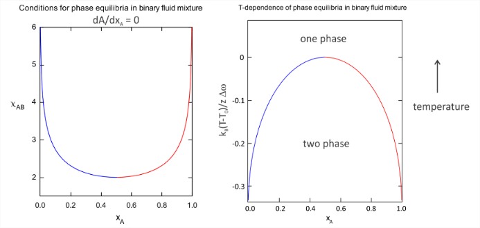
Note that 50/50 mixtures with \(2 < \chi_{AB} < 2.8\) have a negative free energy of mixing to create a single homogeneous phase, yet, the system can still lower the free energy further by phase separating. As seen in the figure, \(\chi_{AB} = 2\) marks a crossover from one phase mixtures to two phase mixtures, which is the signature of a critical point. We can find the conditions for phase equilibria by locating the free energy minima as a function of \(\chi_{AB}\), which leads to the phase diagrams as a function of \(\chi_{AB}\) and \(T\) below. The critical temperature for crossover from one- to two-phase behavior is \(T_0\), and \(\Delta \omega\) is the average differential change in interaction energy defined in eq. (\(\ref{eq2.3.10}\)).

Readings

1. K. Dill and S. Bromberg, Molecular Driving Forces: Statistical Thermodynamics in Biology, Chemistry, Physics, and Nanoscience. (Taylor & Francis Group, New York, 2010).
2. W. W. Graessley, Polymeric Liquids and Networks: Structure and Properties. (Garland Science, New York, 2004), Ch. 3.

_____________________________________

1. J. H. Hildebrand and R. L. Scott, Regular Solutions. (Prentice-Hall, Englewood Cliffs, N.J., 1962).