Summary

Last updated
Save as PDF

Page ID: 275455

Contributor
Analytical Sciences Digital Library

\( \newcommand{\vecs}[1]{\overset { \scriptstyle \rightharpoonup} {\mathbf{#1}} } \) \( \newcommand{\vecd}[1]{\overset{-\!-\!\rightharpoonup}{\vphantom{a}\smash {#1}}} \)\(\newcommand{\id}{\mathrm{id}}\) \( \newcommand{\Span}{\mathrm{span}}\) \( \newcommand{\kernel}{\mathrm{null}\,}\) \( \newcommand{\range}{\mathrm{range}\,}\) \( \newcommand{\RealPart}{\mathrm{Re}}\) \( \newcommand{\ImaginaryPart}{\mathrm{Im}}\) \( \newcommand{\Argument}{\mathrm{Arg}}\) \( \newcommand{\norm}[1]{\| #1 \|}\) \( \newcommand{\inner}[2]{\langle #1, #2 \rangle}\) \( \newcommand{\Span}{\mathrm{span}}\) \(\newcommand{\id}{\mathrm{id}}\) \( \newcommand{\Span}{\mathrm{span}}\) \( \newcommand{\kernel}{\mathrm{null}\,}\) \( \newcommand{\range}{\mathrm{range}\,}\) \( \newcommand{\RealPart}{\mathrm{Re}}\) \( \newcommand{\ImaginaryPart}{\mathrm{Im}}\) \( \newcommand{\Argument}{\mathrm{Arg}}\) \( \newcommand{\norm}[1]{\| #1 \|}\) \( \newcommand{\inner}[2]{\langle #1, #2 \rangle}\) \( \newcommand{\Span}{\mathrm{span}}\)\(\newcommand{\AA}{\unicode[.8,0]{x212B}}\)

After completing this module you should more fully understand the importance of considering the population from which a sample is drawn. The population of US pennies is not singular. Our data, which is limited to pennies minted between 1972 and 1992, show that there are two distinct populations and that a change in the composition of a penny must have occurred in 1982. There have been other changes in the penny, such as different designs, so there might be other populations that we have not considered in this module.

Trying to reach a conclusion about the mass of a penny using samples drawn from more than one population leads to an error in our analysis. The mean of 2.769 g reported in Task 1 of Problem 1, which did not consider the year of minting, is meaningless because no single penny can have this mass. For data drawn from a single population that follows a normal distribution (the classic "bell-shaped curve"),

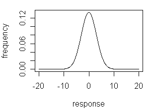
which often is typical of the data we collect in lab, the sample's mean approximates the population's mean and the sample's standard deviation approximates the population's standard deviation.

Another important lesson from this module is the importance of examining your data visually. Much useful information and possibly some surprising trends may be evident in such plots.

Additional information on the topics covered in this module is available for further study, or return to the Data Analysis home page to explore other modules.