
1. Introduction
- Page ID
- 73747

\( \newcommand{\vecs}[1]{\overset { \scriptstyle \rightharpoonup} {\mathbf{#1}} } \)
\( \newcommand{\vecd}[1]{\overset{-\!-\!\rightharpoonup}{\vphantom{a}\smash {#1}}} \)
\( \newcommand{\id}{\mathrm{id}}\) \( \newcommand{\Span}{\mathrm{span}}\)
( \newcommand{\kernel}{\mathrm{null}\,}\) \( \newcommand{\range}{\mathrm{range}\,}\)
\( \newcommand{\RealPart}{\mathrm{Re}}\) \( \newcommand{\ImaginaryPart}{\mathrm{Im}}\)
\( \newcommand{\Argument}{\mathrm{Arg}}\) \( \newcommand{\norm}[1]{\| #1 \|}\)
\( \newcommand{\inner}[2]{\langle #1, #2 \rangle}\)
\( \newcommand{\Span}{\mathrm{span}}\)
\( \newcommand{\id}{\mathrm{id}}\)
\( \newcommand{\Span}{\mathrm{span}}\)
\( \newcommand{\kernel}{\mathrm{null}\,}\)
\( \newcommand{\range}{\mathrm{range}\,}\)
\( \newcommand{\RealPart}{\mathrm{Re}}\)
\( \newcommand{\ImaginaryPart}{\mathrm{Im}}\)
\( \newcommand{\Argument}{\mathrm{Arg}}\)
\( \newcommand{\norm}[1]{\| #1 \|}\)
\( \newcommand{\inner}[2]{\langle #1, #2 \rangle}\)
\( \newcommand{\Span}{\mathrm{span}}\) \( \newcommand{\AA}{\unicode[.8,0]{x212B}}\)
\( \newcommand{\vectorA}[1]{\vec{#1}} % arrow\)
\( \newcommand{\vectorAt}[1]{\vec{\text{#1}}} % arrow\)
\( \newcommand{\vectorB}[1]{\overset { \scriptstyle \rightharpoonup} {\mathbf{#1}} } \)
\( \newcommand{\vectorC}[1]{\textbf{#1}} \)
\( \newcommand{\vectorD}[1]{\overrightarrow{#1}} \)
\( \newcommand{\vectorDt}[1]{\overrightarrow{\text{#1}}} \)
\( \newcommand{\vectE}[1]{\overset{-\!-\!\rightharpoonup}{\vphantom{a}\smash{\mathbf {#1}}}} \)
\( \newcommand{\vecs}[1]{\overset { \scriptstyle \rightharpoonup} {\mathbf{#1}} } \)
\( \newcommand{\vecd}[1]{\overset{-\!-\!\rightharpoonup}{\vphantom{a}\smash {#1}}} \)
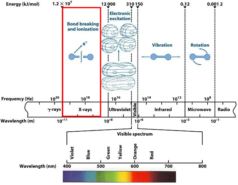
\(\newcommand{\avec}{\mathbf a}\) \(\newcommand{\bvec}{\mathbf b}\) \(\newcommand{\cvec}{\mathbf c}\) \(\newcommand{\dvec}{\mathbf d}\) \(\newcommand{\dtil}{\widetilde{\mathbf d}}\) \(\newcommand{\evec}{\mathbf e}\) \(\newcommand{\fvec}{\mathbf f}\) \(\newcommand{\nvec}{\mathbf n}\) \(\newcommand{\pvec}{\mathbf p}\) \(\newcommand{\qvec}{\mathbf q}\) \(\newcommand{\svec}{\mathbf s}\) \(\newcommand{\tvec}{\mathbf t}\) \(\newcommand{\uvec}{\mathbf u}\) \(\newcommand{\vvec}{\mathbf v}\) \(\newcommand{\wvec}{\mathbf w}\) \(\newcommand{\xvec}{\mathbf x}\) \(\newcommand{\yvec}{\mathbf y}\) \(\newcommand{\zvec}{\mathbf z}\) \(\newcommand{\rvec}{\mathbf r}\) \(\newcommand{\mvec}{\mathbf m}\) \(\newcommand{\zerovec}{\mathbf 0}\) \(\newcommand{\onevec}{\mathbf 1}\) \(\newcommand{\real}{\mathbb R}\) \(\newcommand{\twovec}[2]{\left[\begin{array}{r}#1 \\ #2 \end{array}\right]}\) \(\newcommand{\ctwovec}[2]{\left[\begin{array}{c}#1 \\ #2 \end{array}\right]}\) \(\newcommand{\threevec}[3]{\left[\begin{array}{r}#1 \\ #2 \\ #3 \end{array}\right]}\) \(\newcommand{\cthreevec}[3]{\left[\begin{array}{c}#1 \\ #2 \\ #3 \end{array}\right]}\) \(\newcommand{\fourvec}[4]{\left[\begin{array}{r}#1 \\ #2 \\ #3 \\ #4 \end{array}\right]}\) \(\newcommand{\cfourvec}[4]{\left[\begin{array}{c}#1 \\ #2 \\ #3 \\ #4 \end{array}\right]}\) \(\newcommand{\fivevec}[5]{\left[\begin{array}{r}#1 \\ #2 \\ #3 \\ #4 \\ #5 \\ \end{array}\right]}\) \(\newcommand{\cfivevec}[5]{\left[\begin{array}{c}#1 \\ #2 \\ #3 \\ #4 \\ #5 \\ \end{array}\right]}\) \(\newcommand{\mattwo}[4]{\left[\begin{array}{rr}#1 \amp #2 \\ #3 \amp #4 \\ \end{array}\right]}\) \(\newcommand{\laspan}[1]{\text{Span}\{#1\}}\) \(\newcommand{\bcal}{\cal B}\) \(\newcommand{\ccal}{\cal C}\) \(\newcommand{\scal}{\cal S}\) \(\newcommand{\wcal}{\cal W}\) \(\newcommand{\ecal}{\cal E}\) \(\newcommand{\coords}[2]{\left\{#1\right\}_{#2}}\) \(\newcommand{\gray}[1]{\color{gray}{#1}}\) \(\newcommand{\lgray}[1]{\color{lightgray}{#1}}\) \(\newcommand{\rank}{\operatorname{rank}}\) \(\newcommand{\row}{\text{Row}}\) \(\newcommand{\col}{\text{Col}}\) \(\renewcommand{\row}{\text{Row}}\) \(\newcommand{\nul}{\text{Nul}}\) \(\newcommand{\var}{\text{Var}}\) \(\newcommand{\corr}{\text{corr}}\) \(\newcommand{\len}[1]{\left|#1\right|}\) \(\newcommand{\bbar}{\overline{\bvec}}\) \(\newcommand{\bhat}{\widehat{\bvec}}\) \(\newcommand{\bperp}{\bvec^\perp}\) \(\newcommand{\xhat}{\widehat{\xvec}}\) \(\newcommand{\vhat}{\widehat{\vvec}}\) \(\newcommand{\uhat}{\widehat{\uvec}}\) \(\newcommand{\what}{\widehat{\wvec}}\) \(\newcommand{\Sighat}{\widehat{\Sigma}}\) \(\newcommand{\lt}{<}\) \(\newcommand{\gt}{>}\) \(\newcommand{\amp}{&}\) \(\definecolor{fillinmathshade}{gray}{0.9}\)The Electromagnetic Spectrum
How does light affect molecules and atoms?
D.C. Harris, Quantitative Chemical Analysis, 7th Ed., Freeman, NY, 2007.
X-Ray Interactions With Matter
When X-rays encounter matter, they can be:
- Absorbed or transmitted through the sample (Medical X-Rays – used to see inside materials)

www.seawayort.com/hand.htm
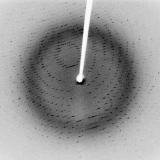
- Diffracted or scattered from an ordered crystal (X-Ray Diffraction – used to study crystal structure)
- Cause the generation of X-rays of different “colors” (X-Ray Fluorescence – used to determine elemental composition)
Atomic Structure
- An atom consists of a nucleus (protons and neutrons) and electrons
- Z is used to represent the atomic number of an element (the number of protons and electrons)
- Electrons spin in shells at specific distances from the nucleus
- Electrons take on discrete (quantized) energy levels (cannot occupy levels between shells
- Inner shell electrons are bound more tightly and are harder to remove from the atom
Adapted from Thermo Scientific Quant’X EDXRF training manual
Electron Shells
Shells have specific names (i.e., K, L, M) and only hold a certain number of electrons
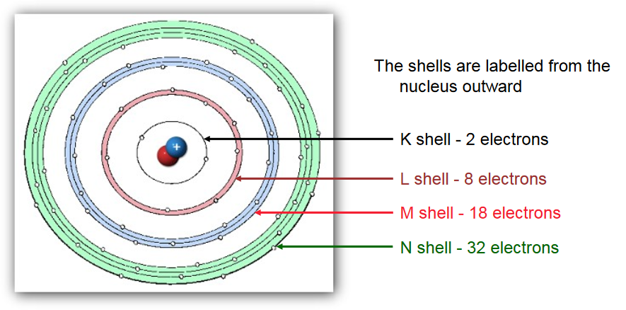
X-rays typically affect only inner shell (K, L) electrons
Adapted from Thermo Scientific Quant’X EDXRF training manual
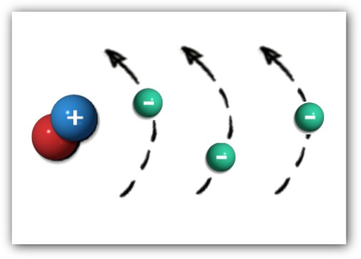
Moving Electrons to/from Shells
Binding Energy versus Potential Energy
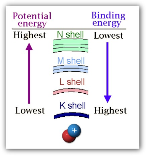
- The K shell has the highest binding energy and hence it takes more energy to remove an electron from a K shell (i.e., high energy X-ray) compared to an L shell (i.e., lower energy X-ray)
- The N shell has the highest potential energy and hence an electron falling from the N shell to the K shell would release more energy (i.e., higher energy X-ray) compared to an L shell (i.e., lower energy X-ray)
Adapted from Thermo Scientific Quant’X EDXRF training manual
XRF – A Physical Description
Step 1: When an X-ray photon of sufficient energy strikes an atom, it dislodges an electron from one of its inner shells (K in this case)
Step 2a: The atom fills the vacant K shell with an electron from the L shell; as the electron drops to the lower energy state, excess energy is released as a Kα X-ray
Step 2b: The atom fills the vacant K shell with an electron from the M shell; as the electron drops to the lower energy state, excess energy is released as a Kβ X-ray
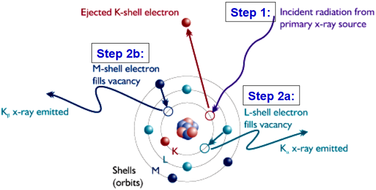
www.niton.com/images/XRF-Excitation-Model.gif
XRF – Sample Analysis
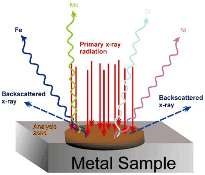
www.niton.com/images/fluoresc...tal-sample.gif
- Since the electronic energy levels for each element are different, the energy of X-ray fluorescence peak can be correlated to a specific element
Simple XRF Spectrum
~10% As in Chinese supplement
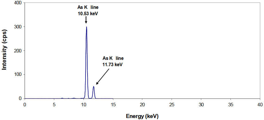
- The presence of As in this sample is confirmed through observation of two peaks centered at energies very close (within ±0.05 keV) to their tabulated (reference) line energies
- These same two peaks will appear in XRF spectra of different arsenic-based materials (i.e., arsenic trioxide, arsenobetaine, etc.)
~10% Pb in imported Mexican tableware
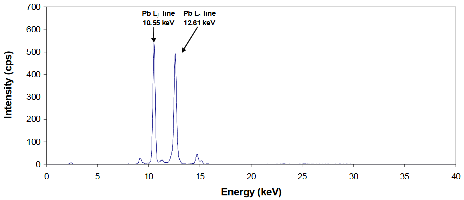
- The presence of Pb in this sample is confirmed through observation of two peaks centered at energies very close (within ±0.05 keV) to their tabulated (reference) line energies
- These same two peaks will appear in XRF spectra of different lead-based materials (i.e., lead arsenate, tetraethyl lead, etc.)
Box Diagram of XRF Instrument
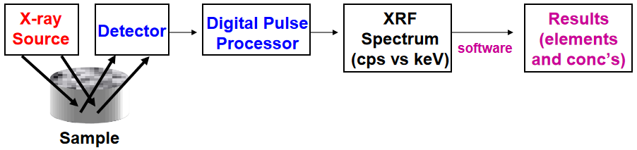
X-ray Source Detector Sample Digital Pulse Processor XRF Spectrum (cps vs keV) Results (elements and conc’s) software
- High energy electrons fired at anode (usually made from Ag or Rh)
Can vary excitation energy from 15-50 kV and current from 10-200 µA
Can use filters to tailor source profile for lower detection limits
- Energy-dispersive multi-channel analyzer – no monochromator needed, Peltiercooled solid state detector monitors both the energy and number of photons over a preset measurement time
The energy of photon in keV is related to the type of element
The emission rate (cps) is related to the concentration of that element
- Concentration of an element determined from factory calibration data, sample thickness as estimated from source backscatter, and other parameters
Different Types of XRF Instruments
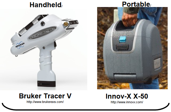
- EASY TO USE (“point and shoot”)
- Used for SCREENING
- Can give ACCURATE RESULTS when used by a knowledgeable operator
- Primary focus of these materials
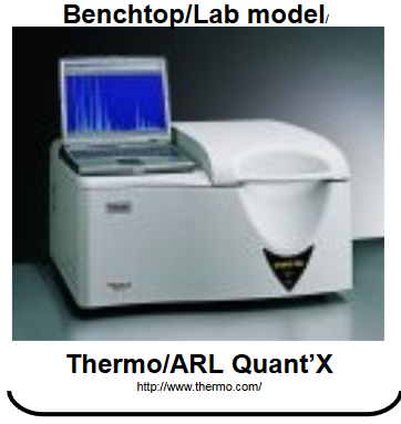
- COMPLEX SOFTWARE
- Used in LAB ANALYSIS
- Designed to give ACCURATE RESULTS
(autosampler, optimized excitation, report generation)