Sampling
- Page ID
- 149072
\( \newcommand{\vecs}[1]{\overset { \scriptstyle \rightharpoonup} {\mathbf{#1}} } \)
\( \newcommand{\vecd}[1]{\overset{-\!-\!\rightharpoonup}{\vphantom{a}\smash {#1}}} \)
\( \newcommand{\dsum}{\displaystyle\sum\limits} \)
\( \newcommand{\dint}{\displaystyle\int\limits} \)
\( \newcommand{\dlim}{\displaystyle\lim\limits} \)
\( \newcommand{\id}{\mathrm{id}}\) \( \newcommand{\Span}{\mathrm{span}}\)
( \newcommand{\kernel}{\mathrm{null}\,}\) \( \newcommand{\range}{\mathrm{range}\,}\)
\( \newcommand{\RealPart}{\mathrm{Re}}\) \( \newcommand{\ImaginaryPart}{\mathrm{Im}}\)
\( \newcommand{\Argument}{\mathrm{Arg}}\) \( \newcommand{\norm}[1]{\| #1 \|}\)
\( \newcommand{\inner}[2]{\langle #1, #2 \rangle}\)
\( \newcommand{\Span}{\mathrm{span}}\)
\( \newcommand{\id}{\mathrm{id}}\)
\( \newcommand{\Span}{\mathrm{span}}\)
\( \newcommand{\kernel}{\mathrm{null}\,}\)
\( \newcommand{\range}{\mathrm{range}\,}\)
\( \newcommand{\RealPart}{\mathrm{Re}}\)
\( \newcommand{\ImaginaryPart}{\mathrm{Im}}\)
\( \newcommand{\Argument}{\mathrm{Arg}}\)
\( \newcommand{\norm}[1]{\| #1 \|}\)
\( \newcommand{\inner}[2]{\langle #1, #2 \rangle}\)
\( \newcommand{\Span}{\mathrm{span}}\) \( \newcommand{\AA}{\unicode[.8,0]{x212B}}\)
\( \newcommand{\vectorA}[1]{\vec{#1}} % arrow\)
\( \newcommand{\vectorAt}[1]{\vec{\text{#1}}} % arrow\)
\( \newcommand{\vectorB}[1]{\overset { \scriptstyle \rightharpoonup} {\mathbf{#1}} } \)
\( \newcommand{\vectorC}[1]{\textbf{#1}} \)
\( \newcommand{\vectorD}[1]{\overrightarrow{#1}} \)
\( \newcommand{\vectorDt}[1]{\overrightarrow{\text{#1}}} \)
\( \newcommand{\vectE}[1]{\overset{-\!-\!\rightharpoonup}{\vphantom{a}\smash{\mathbf {#1}}}} \)
\( \newcommand{\vecs}[1]{\overset { \scriptstyle \rightharpoonup} {\mathbf{#1}} } \)
\(\newcommand{\longvect}{\overrightarrow}\)
\( \newcommand{\vecd}[1]{\overset{-\!-\!\rightharpoonup}{\vphantom{a}\smash {#1}}} \)
\(\newcommand{\avec}{\mathbf a}\) \(\newcommand{\bvec}{\mathbf b}\) \(\newcommand{\cvec}{\mathbf c}\) \(\newcommand{\dvec}{\mathbf d}\) \(\newcommand{\dtil}{\widetilde{\mathbf d}}\) \(\newcommand{\evec}{\mathbf e}\) \(\newcommand{\fvec}{\mathbf f}\) \(\newcommand{\nvec}{\mathbf n}\) \(\newcommand{\pvec}{\mathbf p}\) \(\newcommand{\qvec}{\mathbf q}\) \(\newcommand{\svec}{\mathbf s}\) \(\newcommand{\tvec}{\mathbf t}\) \(\newcommand{\uvec}{\mathbf u}\) \(\newcommand{\vvec}{\mathbf v}\) \(\newcommand{\wvec}{\mathbf w}\) \(\newcommand{\xvec}{\mathbf x}\) \(\newcommand{\yvec}{\mathbf y}\) \(\newcommand{\zvec}{\mathbf z}\) \(\newcommand{\rvec}{\mathbf r}\) \(\newcommand{\mvec}{\mathbf m}\) \(\newcommand{\zerovec}{\mathbf 0}\) \(\newcommand{\onevec}{\mathbf 1}\) \(\newcommand{\real}{\mathbb R}\) \(\newcommand{\twovec}[2]{\left[\begin{array}{r}#1 \\ #2 \end{array}\right]}\) \(\newcommand{\ctwovec}[2]{\left[\begin{array}{c}#1 \\ #2 \end{array}\right]}\) \(\newcommand{\threevec}[3]{\left[\begin{array}{r}#1 \\ #2 \\ #3 \end{array}\right]}\) \(\newcommand{\cthreevec}[3]{\left[\begin{array}{c}#1 \\ #2 \\ #3 \end{array}\right]}\) \(\newcommand{\fourvec}[4]{\left[\begin{array}{r}#1 \\ #2 \\ #3 \\ #4 \end{array}\right]}\) \(\newcommand{\cfourvec}[4]{\left[\begin{array}{c}#1 \\ #2 \\ #3 \\ #4 \end{array}\right]}\) \(\newcommand{\fivevec}[5]{\left[\begin{array}{r}#1 \\ #2 \\ #3 \\ #4 \\ #5 \\ \end{array}\right]}\) \(\newcommand{\cfivevec}[5]{\left[\begin{array}{c}#1 \\ #2 \\ #3 \\ #4 \\ #5 \\ \end{array}\right]}\) \(\newcommand{\mattwo}[4]{\left[\begin{array}{rr}#1 \amp #2 \\ #3 \amp #4 \\ \end{array}\right]}\) \(\newcommand{\laspan}[1]{\text{Span}\{#1\}}\) \(\newcommand{\bcal}{\cal B}\) \(\newcommand{\ccal}{\cal C}\) \(\newcommand{\scal}{\cal S}\) \(\newcommand{\wcal}{\cal W}\) \(\newcommand{\ecal}{\cal E}\) \(\newcommand{\coords}[2]{\left\{#1\right\}_{#2}}\) \(\newcommand{\gray}[1]{\color{gray}{#1}}\) \(\newcommand{\lgray}[1]{\color{lightgray}{#1}}\) \(\newcommand{\rank}{\operatorname{rank}}\) \(\newcommand{\row}{\text{Row}}\) \(\newcommand{\col}{\text{Col}}\) \(\renewcommand{\row}{\text{Row}}\) \(\newcommand{\nul}{\text{Nul}}\) \(\newcommand{\var}{\text{Var}}\) \(\newcommand{\corr}{\text{corr}}\) \(\newcommand{\len}[1]{\left|#1\right|}\) \(\newcommand{\bbar}{\overline{\bvec}}\) \(\newcommand{\bhat}{\widehat{\bvec}}\) \(\newcommand{\bperp}{\bvec^\perp}\) \(\newcommand{\xhat}{\widehat{\xvec}}\) \(\newcommand{\vhat}{\widehat{\vvec}}\) \(\newcommand{\uhat}{\widehat{\uvec}}\) \(\newcommand{\what}{\widehat{\wvec}}\) \(\newcommand{\Sighat}{\widehat{\Sigma}}\) \(\newcommand{\lt}{<}\) \(\newcommand{\gt}{>}\) \(\newcommand{\amp}{&}\) \(\definecolor{fillinmathshade}{gray}{0.9}\)At the end of this assignment students will be able to:
- Define various sampling strategies.
- Assess the benefits and limitations of different sampling strategies.
- Determine an appropriate sampling plan for an analysis.
An important aspect of designing an experiment is collecting a representative sample. What is a representative sample? That is often a tough question to answer. It is important to ensure samples are representative for the analyte of interest. If sampling is not done correctly it could be the “weak link” in an analysis, leading to inaccurate results. Often, sampling can be a source of error that is overlooked.
Purpose
The purpose of this assignment is to address questions related to designing a sampling plan.
Designing a Sampling Plan
The key questions which must be considered are:
1. From where within the target population should we collect samples?
2. What type of samples should we collect?
3. What is the minimum amount of sample for each analysis?
4. How many samples should we analyze?
5. How can we minimize the overall variance for the analysis?

Map of
Where to Sample?
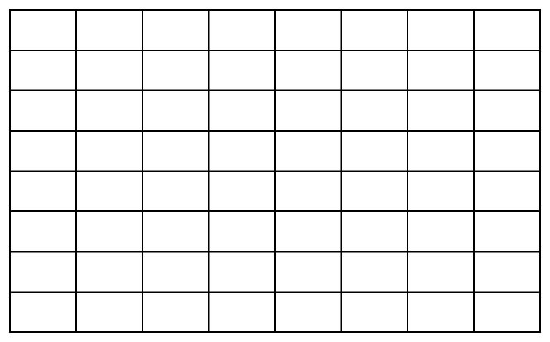
How do you obtain a representative sample? One approach is to take a grab sample. Consider a solid sample divided out as a grid, below. How do you choose where to grab from? One approach is to choose randomly.
Q1. For any given analysis you would have multiple samples for validation of results. Assume you would like eight grab samples of the solid to be evaluated. Pick eight random grab samples from the solid sample divided as a grid below. How do you ensure your sampling of the solid is random?
Now take a look at the following solid samples divided into grids with the location of the analyte of interest (within the solid sample) identified (colored squares).
A
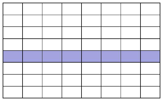
B
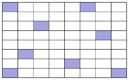
Q2. Would you consider the samples above to be heterogeneous or homogeneous?
Q3. Did your random sampling (Question 1) affect the potential accuracy or precision of your measurement of the analyte for the samples in grid A or grid B? If so how?
Although we would like to assume that a sample is homogenous it is often not. When trying to sample a heterogeneous sample, you need to consider both distributional and constitutional heterogeneity.
- Distribution heterogeneity is caused by segregation of the sample (i.g. settling).
- Constitutional heterogeneity is a fundamental property of a material and is caused by differences in particle size and/or composition.
Q4. Each of the previous grids is an example of one of these cases. Can you identify which sample is which?
Q5. How does distribution heterogeneity affect accuracy and precision?
Q6. How does constitutional heterogeneity affect accuracy and precision?
Q7. Do you see a scenario where distribution heterogeneity could be magnified by mixing and/or sampling?
If samples are mixed well, distributional heterogeneity is insignificant and only constitutional heterogeneity is present. It is important to note, however, that the analyte’s spatial or temporal distribution might also be of importance in the analysis and mixing may not always be the best choice. For example, maybe you are interested in the amount of heavy metals in sediment samples, but are also interested in how far into the sediment the metals have leached. This would be a case where mixing would not be appropriate.
Types of Sampling Plans:
What we have highlighted above is an example of random sampling, which is often applied to a grid design as shown above. Random sampling strategies can be applied to any target population (i.e. evaluating a solid sample or determining the presence of pesticides in the water of
- Selective (Judgmental) Sampling - this is at the opposite extreme of random sampling, and is done if you have prior information about the target. For example, if you wanted to evaluate the metal content in pennies you may not select coins that are corroded or choose coins from a specific mint date.
- Systematic Sampling - Sampling the target population at regular intervals in space or time. This is often considered to fall between the extremes of random and selective sampling.
- Stratified Sampling – The population may be divided into sub populations (groups) that are distinctly different (this might be size of sample, type of sample, depth of sample). Then, the overall sampling within the groups is randomly conducted and the samples are pooled.
- Cluster sampling- is a sampling technique where the population is divided into groups or clusters and random samples are selected from the cluster for analysis. The main objective of cluster sampling is to reduce costs by increasing sampling efficiency.
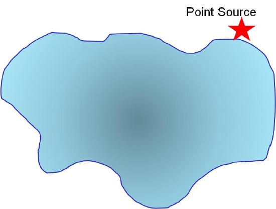
Q8. What is the advantage of implementing a judgmental sampling scheme over random sampling if one knows the point source for the discharge an analyte into a system?
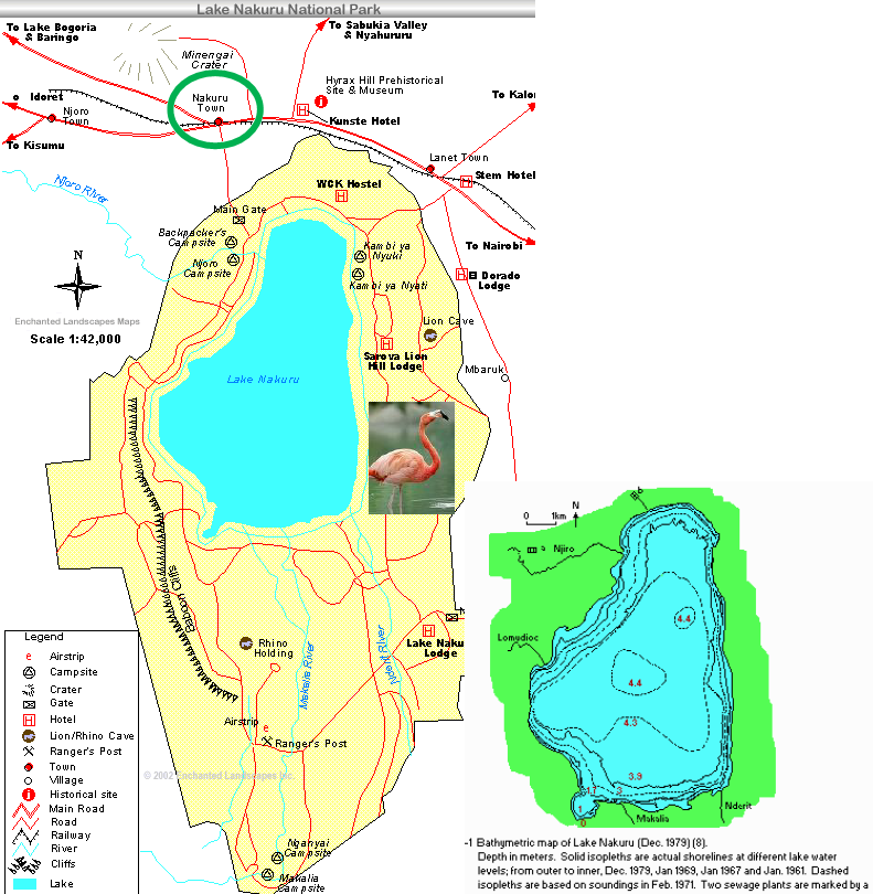
Q9. Assume you have a chosen a selective sampling plan to evaluate pollution from a point source into a lake. Use the diagram below and words to describe your sampling plan.
Q10. Use a grid design (as we have previously done) to show how you would conduct systematic sampling of the pollutant. Is there an advantage to what you might learn using this sampling method? What are the disadvantage(s)?
Q11. Describe how stratified sampling might be applied to evaluate the pollutant in the lake? In general, what is the advantage of stratified sampling over cluster sampling?
Q12. What is a general rule with regard to sampling times or locations to increase the likelihood that samples will be representative?
What Type of Sample to Collect?
When implementing a sample plan often grab samples are used. In some cases composite sampling (combining a set of grab samples into one sample) is more useful. This strategy may be used if:
- There is interest in the target population’s average composition over time and space.
- A single sample does not supply sufficient material for analysis.
Q13. What is the main disadvantage of grab and composite samples?
Q14. Can you think of any control studies you might want to do, when compositing samples?
Q15. Does the EPA Method 525.2 suggest a particular sampling method?
Minimizing Variance - What is the Minimum Amount of Sample? How Many Samples are Needed?
When sampling you want to make sure the sample is not too small, so that the composition is not substantially different from the target population. You also want to ensure you collect an appropriate number of samples for an analysis.
The variance of the (1) analysis method and (2) sampling approach both contribute to the variance in a given analysis. Sampling variance can be improved by collecting more samples of the proper size. Increasing the number of times a sample is analyzed improves the method’s variance.
Q16. What sample size does EPA Method 525.2 suggest for analysis of pesticides in water? Why?
Q17. An analytical method has a percent relative sampling variance of 0.10% and a percent relative method variance of 0.20%. The cost of collecting a sample is $20 and the cost of analyzing a sample is $50. Propose a sampling strategy that provides a maximum percent relative error of ±0.50% (a = 0.05) and a maximum cost of $700.
For further discussion on sampling amounts see section 7.2 in
Design Your Sampling Plan
Of course we would like to collect as many samples as possible to minimize our variance. However, in every lab there are limitations such as those above, related to cost per-sample collected and cost-per analysis.
Q18. The autosampler on the GC-MS you will be using for pesticide analysis has 200 vial locations. How will you choose your representative samples? Below is a picture of Lake Nakuru. Design your sampling plan. Think about random, systematic, clustering, etc. sample strategies. Will you take grab samples or pool samples together?
Helpful Resources
Harvey, D. Chapter 7, Collecting and Preparing Samples.


