Further Study

Last updated
Save as PDF

Page ID: 275466

Contributor
Analytical Sciences Digital Library

\( \newcommand{\vecs}[1]{\overset { \scriptstyle \rightharpoonup} {\mathbf{#1}} } \) \( \newcommand{\vecd}[1]{\overset{-\!-\!\rightharpoonup}{\vphantom{a}\smash {#1}}} \)\(\newcommand{\id}{\mathrm{id}}\) \( \newcommand{\Span}{\mathrm{span}}\) \( \newcommand{\kernel}{\mathrm{null}\,}\) \( \newcommand{\range}{\mathrm{range}\,}\) \( \newcommand{\RealPart}{\mathrm{Re}}\) \( \newcommand{\ImaginaryPart}{\mathrm{Im}}\) \( \newcommand{\Argument}{\mathrm{Arg}}\) \( \newcommand{\norm}[1]{\| #1 \|}\) \( \newcommand{\inner}[2]{\langle #1, #2 \rangle}\) \( \newcommand{\Span}{\mathrm{span}}\) \(\newcommand{\id}{\mathrm{id}}\) \( \newcommand{\Span}{\mathrm{span}}\) \( \newcommand{\kernel}{\mathrm{null}\,}\) \( \newcommand{\range}{\mathrm{range}\,}\) \( \newcommand{\RealPart}{\mathrm{Re}}\) \( \newcommand{\ImaginaryPart}{\mathrm{Im}}\) \( \newcommand{\Argument}{\mathrm{Arg}}\) \( \newcommand{\norm}[1]{\| #1 \|}\) \( \newcommand{\inner}[2]{\langle #1, #2 \rangle}\) \( \newcommand{\Span}{\mathrm{span}}\)\(\newcommand{\AA}{\unicode[.8,0]{x212B}}\)

Descriptive Statistics

In addition to the mean and standard deviation, there are other useful descriptive statistics for characterizing a data set. The median, for, example, is an alternative to the mean as a measure of a data set's central tendency. The median is found by ordering the data from the smallest-to-largest value and reporting the value in the middle. For a data set with an odd number of data points, the median is the middle value (after reordering); thus, for the following data set

3.086, 3.090, 3.097, 3.103, 3.088

the reordered values are

3.086, 3.088, 3.090, 3.097, 3.103

and the median is the third value, or 3.090. For a data set with an even number of data points, the median is the average of the middle two values (after reordering); thus, for the following data set

2.521, 2.511, 2.530, 2.506, 2.487, 2.532

the reordered values are

2.487, 2.506, 2.511, 2.521, 2.530, 2.532

and the median is the average of 2.511 and 2.521, or 2.516.

The range, which is the difference between the largest and smallest values in a data set, provides an alternative to the standard deviation as a measure of the variability in the data set. For example, the range for the two data sets shown above are 0.017 and 0.045, respectively.

Return to Data Set 1 and report the median and range for the 32 pennies.

Follow this link for a further discussion of descriptive statistics. This link provides instructions on using Excel to report descriptive statistics. An on-line calculator can be accessed here.

Alternative Plots

A scatterplot is one of several ways to display data graphically. Other useful plots are boxplots and histograms. This site provides a very brief introduction to these plots. The link on the site to "Questions on this subject" provides you with an opportunity to view boxplots, histograms and summary statistics for a data set consisting of 19 properties for 120 organic molecules. Experiment with creating different plots of the data. This site provides instructions for creating boxplots in Excel.

Normal Distributions

The summary to this module notes that the data we collect in lab typically follows a normal distribution (the classic "bell-shaped curve").

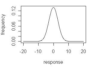
It is not intuitively obvious, however, that this is true. The applet at this site demonstrates that regardless of the shape of the underlying population's distribution, a normal distribution occurs if we gather samples of sufficient size.

Population 1, for example, consists of 101 possible responses (0, 1, 2, ..., 98, 99, 100) each of which is equally probable. The mean for the data set is 50.0. Set the sample size to 1, which means that we will draw one sample at random from this population, record its value and then continue in this fashion. Click on the Draw button and note that the distribution for the results is similar to the distribution for the underlying population and that the mean is approximately 50.

Next, set the sample size to 2, which means that we will draw two samples from the population and record their average. Click on the Draw button and note that the distribution for the results no longer looks like the distribution for the underlying population, but that the mean value continues to be approximately 50. Repeat using sample sizes of 3, 4 and 5 and note how the distribution for results increasingly takes on the shape of a normal distribution. Try using some of the other distributions as well.

The tendency of results to approximate a normal distribution when using large samples is known as the Central Limit Theorem. The samples we analyze in lab generally contain large numbers of individual particles. Consider, for example, a sample of soil, which is not a single particle, but a complex mixture of many individual particles. When determining the concentration of Pb in a soil sample, the result that we report is the average of the amount of Pb in each particle. The large number of particles in a single soil sample tends to favor a normal distribution for our results.

You should be aware that there are other types of distributions for data, such as the binomial and Poisson distributions, but they are less commonly encountered.