34.5: Measuring Particle Size Using Light Scattering

The blue color of the sky during the day and the red color of the sun at sunset are the result of light scattered by small particles of dust, molecules of water, and other gases in the atmosphere. The efficiency of a photon’s scattering depends on its wavelength. We see the sky as blue during the day because violet and blue light scatter to a greater extent than other, longer wavelengths of light. For the same reason, the sun appears red at sunset because red light is less efficiently scattered and is more likely to pass through the atmosphere than other wavelengths of light. The scattering of radiation has been studied since the late 1800s, with applications beginning soon thereafter. The earliest quantitative applications of scattering, which date from the early 1900s, used the elastic scattering of light by colloidal suspensions to determine the concentration of colloidal particles.

Origin of Scattering

If we send a focused, monochromatic beam of radiation with a wavelength \(\lambda\) through a medium of particles with dimensions \(< 1.5 \lambda\), the radiation scatters in all directions. For example, visible radiation of 500 nm is scattered by particles as large as 750 nm in the longest dimension. Two general categories of scattering are recognized. In elastic scattering, radiation is first absorbed by the particles and then emitted without undergoing a change in the radiation’s energy. When the radiation emerges with a change in energy, the scattering is inelastic. Only elastic scattering is considered in this chapter.

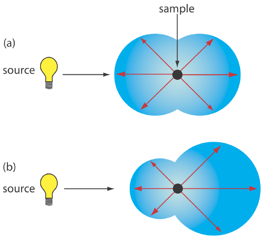
Elastic scattering is divided into two types: Rayleigh, or small-particle scattering, and large-particle scattering. Rayleigh scattering occurs when the scattering particle’s largest dimension is less than 5% of the radiation’s wavelength. The intensity of the scattered radiation is proportional to its frequency to the fourth power, \(\nu^4\)—which accounts for the greater scattering of blue light than red light—and is distributed symmetrically (Figure 34.5.1 a). For larger particles, scattering increases in the forward direction and decreases in the backward direction as the result of constructive and destructive interferences (Figure 34.5.1 b).

Figure \(\PageIndex{1}\). Distribution of radiation for (a) Rayleigh, or small-particle scattering, and (b) large-particle scattering.

Rayleigh Scattering

Small particle, or Rayleigh scattering, measured at an angle of \(\theta\) is the ratio of the intensity of the scattered light, \(I\), to the intensity of the light source, \(I_o\), and is expressed as

\[R_{\theta} = \frac{I}{I_o} = K r^6 \nonumber \]

where \(r_0\) is the radius of the particle and \(K\) is a constant that is a function of the angle of scattering, the wavelength of light used, the refractive index of the particle, and the distance to the particle, \(R\).

Dynamic Light Scattering

In dynamic light scattering (DLS), we use a laser as a light source (see Figure \(\PageIndex{2}\) for an illustration). When the light from the source reaches the sample, which is in a sample cell, it scatters in all directions, as shown in Figure \(\PageIndex{1}\).

Figure \(\PageIndex{2}\). Basic set-up for a DLS experiment. To avoid saturating the detector, the light from the laser is attenuated before entering the sample cell. 

A detector is placed at a fixed angle to collect the light that scatters at that angle. The resulting intensity of scattered light is measure as a function of time. Because the particles in the sample are moving due to Brownian motion, the intensity of light varies with time yielding a noisy signal. Smaller particles diffuse more rapidly than larger particles, which means that fluctuations in intensity with a small particle occurs more rapidly than for a large particle, as seen in Figure \(\PageIndex{3}\).

Figure \(\PageIndex{3}\): The time-dependent intensity of scattered light for (top) large particles and for (bottom) small particles.

To process the data in DLS, we examine the correlation of the signal with itself over small increments of time. This is accomplished by shifting the signal by a small amount (we call this the delay time, \(\tau\)) and computing the correlation between the original signal and the delayed signal. For short delay times, the correlation in intensities is close to 1 because the particles have not had time to move, and for longer delay times the correlation in intensities is close to 0 because the particles have moved significantly; in between these limits, the correlation undergoes an exponential decay. Figure \(\PageIndex{4}\) shows examples of the resulting correlograms for large particles and for small particles. The correlation function, \(G(\tau)\), is defined as

\[G(\tau) = A[1 + Be^{-2 \Gamma \tau}] \label{gtau} \]

The terms \(A\) and \(B\) are, respectively, the baseline and the intercept of the correlation function, and \(\Gamma = Dq^2\), where \(D\) is the translational diffusion coefficient and where \(q\) is equivalent to \((4 \pi n/ \lambda_0) sin(\theta/2)\) where \(n\) is the refractive index, \(\lambda_0\) is the wavelength of the laser, and \(\theta\) is the angle at which scattered light is collected. The relationship between the size of the particles and the translational diffusion coefficient is give by the Stokes-Einstein equation

\[d = \frac{kT}{3 \pi \eta D} \nonumber \]

where \(k\) is Boltzmann's constant, \(T\) is the absolute temperature, and \(\eta\) is the viscosity. Fitting one or more equations for \(G(\tau)\) to the correlogram yields the distribution of particle sizes.

Figure \(\PageIndex{4}\): Correlograms for (a) large and for (b) small particles.

Static Light Scattering

In dynamic light scattering we are interested in how the intensity of scattering changes with time; in static light scattering, we are interested in how the average intensity of scattered light varies with the concentration of particles, \(c\), and the angle, \(\theta\), at which scattering is measured. The extent of scattering, \(R_{\theta}\), for each combination of \(c\) and \(\theta\) is plotted as \(K c / R_{\theta}\), where \(K\) is a constant that is a function of the solvent's refractive index, the change in refracative index with concentration, and Avogadro's number as a function of the angle; the value of \(S\) for the x-axis is chosen to maintain a separation between the data. A typical plot, which is known as a Zimm plot, is shown in Figure \(\PageIndex{5}\).

Figure \(\PageIndex{5}\). Zimm plot used to determine the size and molecular weight of particles. Data is collected using concentrations and angles shown in brown. Extrapolating the data to a concentration of zero (dashed green lines) and a scattering angle of zero (dashed blue lines) yields the solid blue and solid green lines that, in turn, yield values for the molecular weight, \(M\), and particle size, \(R_g\).

Each of the solid brown points gives the value of \(K c / R_{\theta}\) for a combination of concentration and angle. For each angle, the change in \(K c / R_{\theta}\) is extrapolated back to a concentration of zero (the dashed green lines) and for each concentration, the change in \(K c / R_{\theta}\) is extrapolated back to an angle of zero (the dashed blue lines). The resulting extrapolation of \(c_0\) to \(\theta = 0\) gives an intercept that is the inverse of the particles molecular weight, \(M\), and the slope of the extrapolations of \(\theta_0\) to a concentration of zero gives \(R_g\), which is the particle's radius of gyration (it is moving, after all), which is its effective particle size.