22.5: Currents in Electrochemical Cells

Most electrochemical techniques rely on either controlling the current and measuring the resulting potential, or controlling the potential and measuring the resulting current; only potentiometry (see Chapter 23) measures a potential under conditions where there is essentially no current. Understanding the relationship between current, i, and potential, E, is important. Although we learned in Sections 22.3 and 22.4 how to calculated electrode potentials and cell potentials using the Nernst equation, the experimentally measured potentials may differ from their thermodynamic values for a variety of reasons that we outline here.

iR drop

The movement of an electrical charge in an electrochemical cell generates a potential, \(E_{ir}\) defined by Ohm's law

\[E_{ir} = iR \label{ohm} \]

where i is the current and R is the solution's resistance. To account for this, we can include an additional term to the equation for the electrochemical cell's potential

\[E_\text{cell} = E_\text{cathode} - E_\text{anode} - E_{ir} = E_\text{Nernst} - iR \label{cellpot} \]

where \(E_\text{Nernst}\) is the potential from the Nernst equation. The resulting decease in the potential from its idealized value is called the iR drop.

Polarization

Equation \ref{cellpot} indicates that we expect a linear relationship between an electrochemical cell's potential, \(E_\text{cell}\). When this is not the case, the electrochemical cell is said to be polarized. There are several sources that contribute to polarization, which we consider in this section; first, however, we define ideal polarized and nonpolarized electrodes.

Ideal Polarized and Nonpolarized Electrodes and Electrochemical Cells

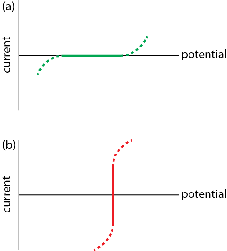
An ideal polarized electrode is one in which a change in potential over a fairly wide range has no effect on the current that flows through the electrode, as we see in Figure \(\PageIndex{1}a\) for the range of potentials defined by the solid green line. Such electrodes are useful because they do not themselves undergo oxidation or reduction—they are electrochemically inert—which makes them a good choice for studying the electrochemical behavior of other species.

An ideal nonpolarized electrode is one in which a change in current has no effect on the electrode's potential, as we see in Figure \(\PageIndex{1}b\) between the limits defined by the solid red line with deviations shown by the dashed red line. Such electrodes are useful because the provided a stable potential against which we can reference the redox potential of other species.

Figure \(\PageIndex{1}\): Current-potential curves for (a) an ideal polarized electrode and for (b) an ideal nonpolarized electrode. For both, the solid line shows the range of (a) potentials or (b) currents where the electrode shows ideal behavior.

Overpotential

The magnitude of polarization when drawing a current is called the overpotential, \(\eta\) and expressed as the difference between the applied potential, E, and the potential from the Nernst equation.

\[\eta = E - E_\text{Nernst} \label{overpot} \]

The overpotential can be subdivided into a variety of sources, a few of which are discussed below.

Concentration Polarization

The reduction of Fe³⁺ to Fe²⁺ in an electrochemical cell consumes an electron, which is drawn from the electrode. The oxidation of another species, perhaps the solvent, at a second electrode is the source of this electron. Because the reduction of Fe³⁺ to Fe²⁺ consumes one electron, the flow of electrons between the electrodes—in other words, the current—is a measure of the rate at which Fe³⁺ is reduced.

The rate of the reaction \(\text{Fe}^{3+}(aq) \rightleftharpoons \text{ Fe}^{2+}(aq) + e^-\) is the change in the concentration of Fe³⁺ as a function of time.

In order for the reduction of Fe³⁺ to Fe²⁺ to take place, Fe³⁺ must move from the bulk solution into the layer of solution immediately adjacent to the electrode and then diffuse to the electrode's surface; this is called the diffusion layer. Once the reduction takes place, the Fe²⁺ produced must diffuse away from the electrode's surface and enter into the bulk solution. These two processes are called mass transfer and if we try to change the electrode's potential too quickly, mass transfer may result in concentrations of Fe³⁺ to Fe²⁺ at the electrode's surface that are different from that in bulk solution, resulting in concentration polarization.

Let's use the reduction of Fe³⁺ to Fe²⁺ at the cathode of a galvanic cell to think though how concentration polarization affects the potential we measure. From the Nernst equation we know that

\[E = E_{\ce{Fe^{3+}}/\ce{Fe^{2+}}}^{\circ} - \frac {0.05916} {1} \log \frac {[\ce{Fe^{2+}}]}{[\ce{Fe^{3+}}]} = +0.771 - \frac {0.05916} {1} \log \frac {[\ce{Fe^{2+}}]}{[\ce{Fe^{3+}}]} \label{iron1} \]

If the mass transfer of Fe³⁺ from bulk solution to the electrode's surface is slow and if mass transfer of Fe²⁺ from the electrode's surface to bulk solution is slow, then the concentration of Fe³⁺ at the electrode's surface is smaller than in bulk solution and the concentration of Fe²⁺ at the electrode's surface is greater than in the bulk solution. As a result, the ratio \(\frac {[\ce{Fe^{2+}}]}{[\ce{Fe^{3+}}]}\) is greater than that predicted by the bulk concentrations of Fe³⁺ and Fe²⁺ and the potential of the cathode is smaller (less positive) than the value +0.771 V predicted by the bulk concentrations of Fe³⁺ and Fe²⁺. The resulting potential of the electrochemical cell

\[E_\text{cell} = E_\text{cathode} - E_\text{anode} \label{iron2} \]

is less positive than that predicted by the bulk concentrations of Fe³⁺ and Fe²⁺ due to this concentration polarization.

Other kinetic processes can contribute to polarization, including the rate of chemical reactions that take place within the layer of solution near the electrode's surface, the kinetics of reactions in which the electroactive species absorb or desorb from the electrode's surface, and the kinetics of the electron transfer process itself. More details on these are included in later chapters covering specific electrochemical techniques.