5.4: Modeling Distributions Using R

Last updated
Save as PDF

Page ID: 219090

$ \newcommand{\vecs}[1]{\overset { \scriptstyle \rightharpoonup} {\mathbf{#1}} } $ $ \newcommand{\vecd}[1]{\overset{-\!-\!\rightharpoonup}{\vphantom{a}\smash {#1}}} $$\newcommand{\id}{\mathrm{id}}$ $ \newcommand{\Span}{\mathrm{span}}$ $ \newcommand{\kernel}{\mathrm{null}\,}$ $ \newcommand{\range}{\mathrm{range}\,}$ $ \newcommand{\RealPart}{\mathrm{Re}}$ $ \newcommand{\ImaginaryPart}{\mathrm{Im}}$ $ \newcommand{\Argument}{\mathrm{Arg}}$ $ \newcommand{\norm}[1]{\| #1 \|}$ $ \newcommand{\inner}[2]{\langle #1, #2 \rangle}$ $ \newcommand{\Span}{\mathrm{span}}$ $\newcommand{\id}{\mathrm{id}}$ $ \newcommand{\Span}{\mathrm{span}}$ $ \newcommand{\kernel}{\mathrm{null}\,}$ $ \newcommand{\range}{\mathrm{range}\,}$ $ \newcommand{\RealPart}{\mathrm{Re}}$ $ \newcommand{\ImaginaryPart}{\mathrm{Im}}$ $ \newcommand{\Argument}{\mathrm{Arg}}$ $ \newcommand{\norm}[1]{\| #1 \|}$ $ \newcommand{\inner}[2]{\langle #1, #2 \rangle}$ $ \newcommand{\Span}{\mathrm{span}}$$\newcommand{\AA}{\unicode[.8,0]{x212B}}$

The base installation of R includes a variety of functions for working with uniform distributions, binomial distributions, Poisson distributions, and normal distributions. These functions come in four forms that take the general form xdist where dist is the type of distribution (unif for a uniform distribution, binom for a binomial distribution, pois for a Poisson distribution, and norm for a normal distribution), and where x defines the information we extract from the distribution. For example, the function dunif()returns the probability of obtaining a specific value drawn from a uniform distribution, the function pbinom() returns the probability of obtaining a result less than a defined value from a binomial distribution, the function qpois() returns the upper boundary that includes a defined percentage of results from a Poisson distribution, and the function rnomr() returns results drawn at random from a normal distribution.

Modeling a Uniform Distribution Using R

When you purchase a Class A 10.00-mL volumetric pipet it comes with a tolerance of ±0.02 mL, which is the manufacturer’s way of saying that the pipet’s true volume is no less than 9.98 mL and no greater than 10.02 mL. Suppose a manufacturer produces 10,000 pipets, how many might we expect to have a volume between 9.990 mL and 9.992 mL? A uniform distribution is the choice when the manufacturer provides a tolerance range without specifying a level of confidence and when there is no reason to believe that results near the center of the range are more likely than results at the ends of the range.

To simulate a uniform distribution we use R’s runif(n, min, max) function, which returns n random values drawn from a uniform distribution defined by its minimum (min) and its maximum (max) limits. The result is shown in Figure $\PageIndex{1}$, where the dots, added using the points()function, show the theoretical uniform distribution at the midpoint of each of the histogram’s bins.

# create vector of volumes for 10000 pipets drawn at random from uniform distribution

pipet = runif(10000, 9.98, 10.02)

# create histogram using 20 bins of size 0.002 mL

pipet_hist = hist(pipet, breaks = seq(9.98, 10.02, 0.002), col = c("blue", "lightblue"), ylab = "number of pipets", xlab = "volume of pipet (mL)", main = NULL)

# overlay points showing expected values for uniform distribution

points(pipet_hist$mids, rep(10000/20, 20), pch = 19)

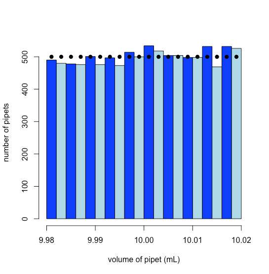
Figure $\PageIndex{1}$: Uniform distribution of volumes for 10000 10-mL volumetric pipets. The individual bars show the simulated results and the individual dots show the expected results.

Saving the histogram to the object pipet_hist allows us to retrieve the number of pipets in each of the histogram’s intervals; thus, there are 476 pipets with volumes between 9.990 mL and 9.992 mL, which is the sixth bar from the left edge of Figure $\PageIndex{1}$.

pipet_hist$counts[6]

[1] 476

Modeling a Binomial Distribution Using R

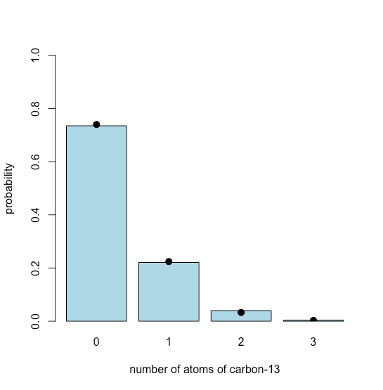
Carbon has two stable, non-radioactive isotopes, ¹²C and ¹³C, with relative isotopic abundances of, respectively, 98.89% and 1.11%. Suppose we are working with cholesterol, C₂₇H₄₄O, which has 27 atoms of carbon. We can use the binomial distribution to model the expected distribution for the number of atoms ¹³C in 1000 cholesterol molecules.

To simulate the distribution we use R’s rbinom(n, size, prob) function, which returns n random values drawn from a binomial distribution defined by the size of our sample, which is the number of possible carbon atoms, and the isotopic abundance of ¹³C, which is itsprobor probability. The result is shown in Figure $\PageIndex{2}$, where the dots, added using the points()function, show the theoretical binomial distribution. These theoretical values are calculated using the dbinom() function. The bar plot is assigned to the object chol_bar to provide access to the values of x when plotting the points.

# create vector with 1000 values drawn at random from binomial distribution

cholesterol = rbinom(1000, 27, 0.0111)

# create bar plot of results; table(cholesterol) determines the number of cholesterol

# molecules with 0, 1, 2... atoms of carbon-13; dividing by 1000 gives probability

chol_bar = barplot(table(cholesterol)/1000, col = "lightblue", ylim = c(0,1), xlab = "number of atoms of carbon-13", ylab = "probability")

# theoretical results for binomial distribution of carbon-13 in cholesterol

chol_binom = dbinom(seq(0,27,1), 27, 0.0111)

# overlay theoretical results for binomial distribution

points(x = chol_bar, y = chol_binom[1:length(chol_bar)], cex = 1.25, pch = 19)

Figure $\PageIndex{2}$: Distribution of results for carbon-13 atoms in cholesterol. The individual bars show the simulated results and the individual dots show the expected results.

Modeling a Poisson Distribution Using R

One measure of the quality of water in lakes used for recreational purposes is a fecal coliform test. In a typical test a sample of water is passed through a membrane filter, which is then placed on a medium to encourage growth of the bacteria and incubated for 24 hours at 44.5°C. The number of colonies of bacteria is reported. Suppose a lake has a natural background level of 5 colonies per 50 mL of water tested and must be closed for swimming if it exceeds 10 colonies per 50 mL of water tested. We can use a Poisson distribution to determine, over the course of a year of daily testing, the probability that a test will exceed this limit even though the lake’s true fecal coliform count remains at its natural background level.

To simulate the distribution we use R’s rpois(n, lambda) function, which returns n random values drawn from a Poisson distribution defined by lambda which is its average incidence. Because we are interested in modeling out a year, n is set to 365 days. The result is shown in Figure $\PageIndex{3}$, where the dots, added using the points() function, shows the theoretical Poisson distribution. These theoretical values are calculated using the dpois() function. The bar plot is assigned to the object choliform_bar to provide access to the values of x when plotting the points.

# create vector of results drawn at random from Poisson distribution

coliforms = rpois(365,5)

# create table of simulated results

coliform_table = table(coliforms)

# create bar plot; ylim ensures there is some space above the plot's highest bar

coliform_bar = barplot(coliform_table, ylim = c(0, 1.2 * max(coliform_table)), col = "lightblue")

# theoretical results for Poisson distribution

d_coliforms = dpois(seq(0,length(coliform_bar) - 1), 5) * 365

# overlay theoretical results for Poisson distribution

points(coliform_bar, d_coliforms, pch = 19)

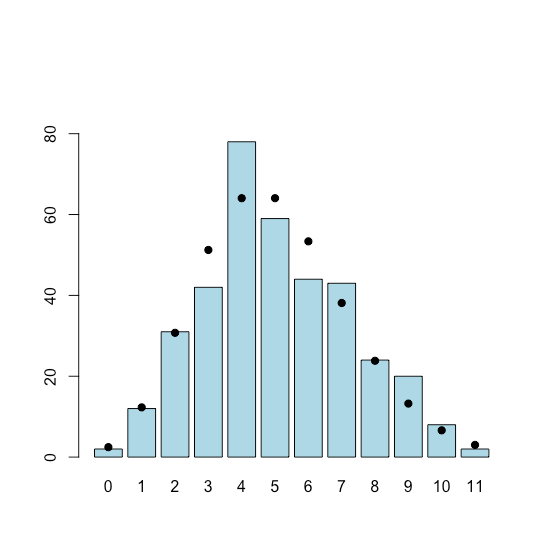
Figure $\PageIndex{3}$: Distribution of results for fecal coliform test over course of a year. The individual bars show the simulated results and the individual dots show the expected results.

To find the number of times our simulated results exceed the limit of 10 coliforms colonies per 50 mL we use R’s which() function to identify within coliforms the values that are greater than 10

coliforms[which(coliforms > 10)]

finding that this happen 2 times over the course of a year.

The theoretical probability that a single test will exceed the limit of 10 colonies per 50 mL of water, we use R’s ppois(q, lambda) function, where q is the value we wish to test, which returns the cumulative probability of obtaining a result less than or equal to q on any day; over the course of 365 days

(1 - ppois(10,5))*365

[1] 4.998773

we expect that on 5 days the fecal coliform count will exceed the limit of 10.

Modeling a Normal Distribution Using R

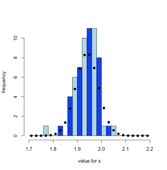
If we place copper metal and an excess of powdered sulfur in a crucible and ignite it, copper sulfide forms with an empirical formula of Cu_xS. The value of x is determined by weighing the Cu and the S before ignition and finding the mass of Cu_xS when the reaction is complete (any excess sulfur leaves as the gas SO₂). The following are the Cu/S ratios from 62 such experiments, of which just 3 are greater than 2. Because of the central limit theorem, we can use a normal distribution to model the data.

Table $\PageIndex{1}$: Experimental Cu/S Ratios When Igniting Cu(s) and S(s).
1.764	1.838	1.890	1.891	1.906	1.908
1.920	1.922	1.936	1.937	1.941	1.942
1.957	1.957	1.963	1.963	1.975	1.976
1.993	1.993	2.029	2.042	1.866	1.872
1.891	1.897	1.899	1.910	1.911	1.916
1.927	1.931	1.935	1.939	1.939	1.940
1.943	1.948	1.953	1.957	1.959	1.962
1.966	1.968	1.969	1.977	1.981	1.981
1.995	1.995	1.865	1.995	1.877	1.900
1.919	1.936	1.941	1.955	1.963	1.973
1.988	2.017

Figure $\PageIndex{4}$ shows the distribution of the experimental results as a histogram overlaid with the theoretical normal distribution calculated assuming that $\mu$ is equal to the mean of the 62 samples and that $\sigma$ is equal to the standard deviation of the 62 samples. Both the experimental data and theoretical normal distribution suggest that most values of x are between 1.85 and 2.03.

# enter the data into a vector with the name cuxs

cuxs = c(1.764, 1.920, 1.957, 1.993, 1.891, 1.927, 1.943, 1.966, 1.995, 1.919, 1.988, 1.838, 1.922, 1.957, 1.993, 1.897, 1.931, 1.948, 1.968, 1.995, 1.936, 2.017, 1.890, 1.936, 1.963, 2.029, 1.899, 1.935, 1.953, 1.969, 1.865, 1.941, 1.891, 1.937, 1.963, 2.042, 1.910, 1.939, 1.957, 1.977, 1.995, 1.955, 1.906, 1.941, 1.975, 1.866, 1.911, 1.939, 1.959, 1.981, 1.877, 1.963, 1.908, 1.942, 1.976, 1.872, 1.916, 1.940, 1.962, 1.981, 1.900, 1.973)

# sequence of ratios over which to display experimental results and theoretical distribution

x = seq(1.7,2.2,0.02)

# create histogram for experimental results

cuxs_hist = hist(cuxs, breaks = x, col = c("blue", "lightblue"), xlab = "value for x", ylab = "frequency", main = NULL)

# calculate theoretical results for normal distribution using the mean and the standard deviation

# for the 62 samples as predictors for mu and sigma

cuxs_theo = dnorm(cuxs_hist$mids, mean = mean(cuxs), sd = sd(cuxs))

# overlay results for theoretical normal distribution

points(cuxs_hist$mids, cuxs_theo, pch = 19)

Figure $\PageIndex{4}$: Distribution of results for ratio of Cu-to-S in preparations of copper sulfide. The individual bars show the simulated results and the individual dots show the expected results.