
4.4: The Distribution of Measurements and Results
- Page ID
- 127559

\( \newcommand{\vecs}[1]{\overset { \scriptstyle \rightharpoonup} {\mathbf{#1}} } \)
\( \newcommand{\vecd}[1]{\overset{-\!-\!\rightharpoonup}{\vphantom{a}\smash {#1}}} \)
\( \newcommand{\id}{\mathrm{id}}\) \( \newcommand{\Span}{\mathrm{span}}\)
( \newcommand{\kernel}{\mathrm{null}\,}\) \( \newcommand{\range}{\mathrm{range}\,}\)
\( \newcommand{\RealPart}{\mathrm{Re}}\) \( \newcommand{\ImaginaryPart}{\mathrm{Im}}\)
\( \newcommand{\Argument}{\mathrm{Arg}}\) \( \newcommand{\norm}[1]{\| #1 \|}\)
\( \newcommand{\inner}[2]{\langle #1, #2 \rangle}\)
\( \newcommand{\Span}{\mathrm{span}}\)
\( \newcommand{\id}{\mathrm{id}}\)
\( \newcommand{\Span}{\mathrm{span}}\)
\( \newcommand{\kernel}{\mathrm{null}\,}\)
\( \newcommand{\range}{\mathrm{range}\,}\)
\( \newcommand{\RealPart}{\mathrm{Re}}\)
\( \newcommand{\ImaginaryPart}{\mathrm{Im}}\)
\( \newcommand{\Argument}{\mathrm{Arg}}\)
\( \newcommand{\norm}[1]{\| #1 \|}\)
\( \newcommand{\inner}[2]{\langle #1, #2 \rangle}\)
\( \newcommand{\Span}{\mathrm{span}}\) \( \newcommand{\AA}{\unicode[.8,0]{x212B}}\)
\( \newcommand{\vectorA}[1]{\vec{#1}} % arrow\)
\( \newcommand{\vectorAt}[1]{\vec{\text{#1}}} % arrow\)
\( \newcommand{\vectorB}[1]{\overset { \scriptstyle \rightharpoonup} {\mathbf{#1}} } \)
\( \newcommand{\vectorC}[1]{\textbf{#1}} \)
\( \newcommand{\vectorD}[1]{\overrightarrow{#1}} \)
\( \newcommand{\vectorDt}[1]{\overrightarrow{\text{#1}}} \)
\( \newcommand{\vectE}[1]{\overset{-\!-\!\rightharpoonup}{\vphantom{a}\smash{\mathbf {#1}}}} \)
\( \newcommand{\vecs}[1]{\overset { \scriptstyle \rightharpoonup} {\mathbf{#1}} } \)
\( \newcommand{\vecd}[1]{\overset{-\!-\!\rightharpoonup}{\vphantom{a}\smash {#1}}} \)
\(\newcommand{\avec}{\mathbf a}\) \(\newcommand{\bvec}{\mathbf b}\) \(\newcommand{\cvec}{\mathbf c}\) \(\newcommand{\dvec}{\mathbf d}\) \(\newcommand{\dtil}{\widetilde{\mathbf d}}\) \(\newcommand{\evec}{\mathbf e}\) \(\newcommand{\fvec}{\mathbf f}\) \(\newcommand{\nvec}{\mathbf n}\) \(\newcommand{\pvec}{\mathbf p}\) \(\newcommand{\qvec}{\mathbf q}\) \(\newcommand{\svec}{\mathbf s}\) \(\newcommand{\tvec}{\mathbf t}\) \(\newcommand{\uvec}{\mathbf u}\) \(\newcommand{\vvec}{\mathbf v}\) \(\newcommand{\wvec}{\mathbf w}\) \(\newcommand{\xvec}{\mathbf x}\) \(\newcommand{\yvec}{\mathbf y}\) \(\newcommand{\zvec}{\mathbf z}\) \(\newcommand{\rvec}{\mathbf r}\) \(\newcommand{\mvec}{\mathbf m}\) \(\newcommand{\zerovec}{\mathbf 0}\) \(\newcommand{\onevec}{\mathbf 1}\) \(\newcommand{\real}{\mathbb R}\) \(\newcommand{\twovec}[2]{\left[\begin{array}{r}#1 \\ #2 \end{array}\right]}\) \(\newcommand{\ctwovec}[2]{\left[\begin{array}{c}#1 \\ #2 \end{array}\right]}\) \(\newcommand{\threevec}[3]{\left[\begin{array}{r}#1 \\ #2 \\ #3 \end{array}\right]}\) \(\newcommand{\cthreevec}[3]{\left[\begin{array}{c}#1 \\ #2 \\ #3 \end{array}\right]}\) \(\newcommand{\fourvec}[4]{\left[\begin{array}{r}#1 \\ #2 \\ #3 \\ #4 \end{array}\right]}\) \(\newcommand{\cfourvec}[4]{\left[\begin{array}{c}#1 \\ #2 \\ #3 \\ #4 \end{array}\right]}\) \(\newcommand{\fivevec}[5]{\left[\begin{array}{r}#1 \\ #2 \\ #3 \\ #4 \\ #5 \\ \end{array}\right]}\) \(\newcommand{\cfivevec}[5]{\left[\begin{array}{c}#1 \\ #2 \\ #3 \\ #4 \\ #5 \\ \end{array}\right]}\) \(\newcommand{\mattwo}[4]{\left[\begin{array}{rr}#1 \amp #2 \\ #3 \amp #4 \\ \end{array}\right]}\) \(\newcommand{\laspan}[1]{\text{Span}\{#1\}}\) \(\newcommand{\bcal}{\cal B}\) \(\newcommand{\ccal}{\cal C}\) \(\newcommand{\scal}{\cal S}\) \(\newcommand{\wcal}{\cal W}\) \(\newcommand{\ecal}{\cal E}\) \(\newcommand{\coords}[2]{\left\{#1\right\}_{#2}}\) \(\newcommand{\gray}[1]{\color{gray}{#1}}\) \(\newcommand{\lgray}[1]{\color{lightgray}{#1}}\) \(\newcommand{\rank}{\operatorname{rank}}\) \(\newcommand{\row}{\text{Row}}\) \(\newcommand{\col}{\text{Col}}\) \(\renewcommand{\row}{\text{Row}}\) \(\newcommand{\nul}{\text{Nul}}\) \(\newcommand{\var}{\text{Var}}\) \(\newcommand{\corr}{\text{corr}}\) \(\newcommand{\len}[1]{\left|#1\right|}\) \(\newcommand{\bbar}{\overline{\bvec}}\) \(\newcommand{\bhat}{\widehat{\bvec}}\) \(\newcommand{\bperp}{\bvec^\perp}\) \(\newcommand{\xhat}{\widehat{\xvec}}\) \(\newcommand{\vhat}{\widehat{\vvec}}\) \(\newcommand{\uhat}{\widehat{\uvec}}\) \(\newcommand{\what}{\widehat{\wvec}}\) \(\newcommand{\Sighat}{\widehat{\Sigma}}\) \(\newcommand{\lt}{<}\) \(\newcommand{\gt}{>}\) \(\newcommand{\amp}{&}\) \(\definecolor{fillinmathshade}{gray}{0.9}\)Earlier we reported results for a determination of the mass of a circulating United States penny, obtaining a mean of 3.117 g and a standard deviation of 0.051 g. Table 4.4.1 shows results for a second, independent determination of a penny’s mass, as well as the data from the first experiment. Although the means and standard deviations for the two experiments are similar, they are not identical. The difference between the two experiments raises some interesting questions. Are the results for one experiment better than the results for the other experiment? Do the two experiments provide equivalent estimates for the mean and the standard deviation? What is our best estimate of a penny’s expected mass? To answer these questions we need to understand how we might predict the properties of all pennies using the results from an analysis of a small sample of pennies. We begin by making a distinction between populations and samples.
| First Experiment | Second Experiment | ||
|---|---|---|---|
| Penny | Mass (g) | Penny | Mass (g) |
| 1 | 3.080 | 1 | 3.052 |
| 2 | 3.094 | 2 | 3.141 |
| 3 | 3.107 | 3 | 3.083 |
| 4 | 3.056 | 4 | 3.083 |
| 5 | 3.112 | 5 | 3.048 |
| 6 | 3.174 | ||
| 7 | 3.198 | ||
| \(\overline{X}\) | 3.117 | 3.081 | |
| \(s\) | 0.051 | 0.037 | |
Populations and Samples
A population is the set of all objects in the system we are investigating. For the data in Table 4.4.1 , the population is all United States pennies in circulation. This population is so large that we cannot analyze every member of the population. Instead, we select and analyze a limited subset, or sample of the population. The data in Table 4.4.1 , for example, shows the results for two such samples drawn from the larger population of all circulating United States pennies.
Probability Distributions for Populations
Table 4.4.1 provides the means and the standard deviations for two samples of circulating United States pennies. What do these samples tell us about the population of pennies? What is the largest possible mass for a penny? What is the smallest possible mass? Are all masses equally probable, or are some masses more common?
To answer these questions we need to know how the masses of individual pennies are distributed about the population’s average mass. We represent the distribution of a population by plotting the probability or frequency of obtaining a specific result as a function of the possible results. Such plots are called probability distributions.
There are many possible probability distributions; in fact, the probability distribution can take any shape depending on the nature of the population. Fortunately many chemical systems display one of several common probability distributions. Two of these distributions, the binomial distribution and the normal distribution, are discussed in this section.
The Binomial Distribution
The binomial distribution describes a population in which the result is the number of times a particular event occurs during a fixed number of trials. Mathematically, the binomial distribution is defined as
\[P(X, N) = \frac {N!} {X!(N - X)!} \times p^X \times (1 - p)^{N - X} \nonumber\]
where P(X , N) is the probability that an event occurs X times during N trials, and p is the event’s probability for a single trial. If you flip a coin five times, P(2,5) is the probability the coin will turn up “heads” exactly twice.
The term N! reads as N-factorial and is the product \(N \times (N – 1) \times (N – 2) \times \cdots \times 1\). For example, 4! is \(4 \times 3 \times 2 \times 1 = 24\). Your calculator probably has a key for calculating factorials.
A binomial distribution has well-defined measures of central tendency and spread. The expected mean value is
\[\mu = Np \nonumber\]
and the expected spread is given by the variance
\[\sigma^2 = Np(1 - p) \nonumber\]
or the standard deviation.
\[\sigma = \sqrt{Np(1 - p)} \nonumber\]
The binomial distribution describes a population whose members have only specific, discrete values. When you roll a die, for example, the possible values are 1, 2, 3, 4, 5, or 6. A roll of 3.45 is not possible. As shown in Worked Example 4.4.1 , one example of a chemical system that obeys the binomial distribution is the probability of finding a particular isotope in a molecule.
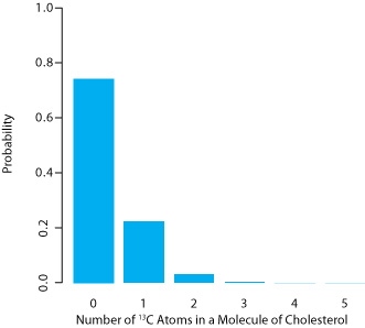
Carbon has two stable, non-radioactive isotopes, 12C and 13C, with relative isotopic abundances of, respectively, 98.89% and 1.11%.
(a) What are the mean and the standard deviation for the number of 13C atoms in a molecule of cholesterol (C27H44O)?
(b) What is the probability that a molecule of cholesterol has no atoms of 13C?
Solution
The probability of finding an atom of 13C in a molecule of cholesterol follows a binomial distribution, where X is the number of 13C atoms, N is the number of carbon atoms in a molecule of cholesterol, and p is the probability that an atom of carbon in 13C.
For (a), the mean number of 13C atoms in a molecule of cholesterol is
\[\mu = Np = 27 \times 0.0111 = 0.300 \nonumber\]
with a standard deviation of
\[\sigma = \sqrt{Np(1 - p)} = \sqrt{27 \times 0.0111 \times (1 - 0.0111)} = 0.544 \nonumber\]
For (b), the probability of finding a molecule of cholesterol without an atom of 13C is
\[P(0, 27) = \frac {27!} {0! \: (27 - 0)!} \times (0.0111)^0 \times (1 - 0.0111)^{27 - 0} = 0.740 \nonumber\]
There is a 74.0% probability that a molecule of cholesterol will not have an atom of 13C, a result consistent with the observation that the mean number of 13C atoms per molecule of cholesterol, 0.300, is less than one.
A portion of the binomial distribution for atoms of 13C in cholesterol is shown in Figure 4.4.1 . Note in particular that there is little probability of finding more than two atoms of 13C in any molecule of cholesterol.
The Normal Distribution
A binomial distribution describes a population whose members have only certain discrete values. This is the case with the number of 13C atoms in cholesterol. A molecule of cholesterol, for example, can have two 13C atoms, but it can not have 2.5 atoms of 13C. A population is continuous if its members may take on any value. The efficiency of extracting cholesterol from a sample, for example, can take on any value between 0% (no cholesterol is extracted) and 100% (all cholesterol is extracted).
The most common continuous distribution is the Gaussian, or normal distribution, the equation for which is
\[f(X) = \frac {1} {\sqrt{2 \pi \sigma^2}} e^{- \frac {(X - \mu)^2} {2 \sigma^2}} \nonumber\]
where \(\mu\) is the expected mean for a population with n members
\[\mu = \frac {\sum_{i = 1}^n X_i} {n} \nonumber\]
and \(\sigma^2\) is the population’s variance.
\[\sigma^2 = \frac {\sum_{i = 1}^n (X_i - \mu)^2} {n} \label{4.1}\]
Examples of three normal distributions, each with an expected mean of 0 and with variances of 25, 100, or 400, respectively, are shown in Figure 4.4.2 . Two features of these normal distribution curves deserve attention. First, note that each normal distribution has a single maximum that corresponds to \(\mu\), and that the distribution is symmetrical about this value. Second, increasing the population’s variance increases the distribution’s spread and decreases its height; the area under the curve, however, is the same for all three distributions.
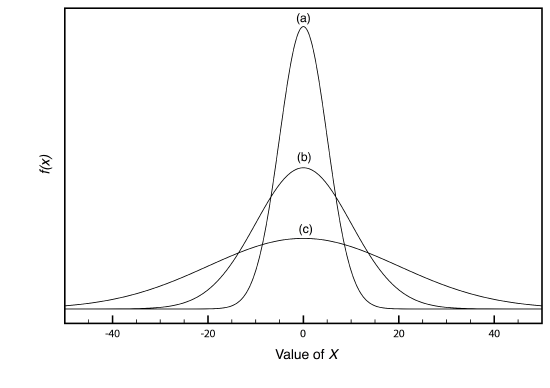
The area under a normal distribution curve is an important and useful property as it is equal to the probability of finding a member of the population within a particular range of values. In Figure 4.4.2 , for example, 99.99% of the population shown in curve (a) have values of X between –20 and +20. For curve (c), 68.26% of the population’s members have values of X between –20 and +20.
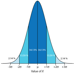
Because a normal distribution depends solely on \(\mu\) and \(\sigma^2\), the probability of finding a member of the population between any two limits is the same for all normally distributed populations. Figure 4.4.3 , for example, shows that 68.26% of the members of a normal distribution have a value within the range \(\mu \pm 1 \sigma\), and that 95.44% of population’s members have values within the range \(\mu \pm 2 \sigma\). Only 0.27% members of a population have values that exceed the expected mean by more than ± 3\(\sigma\). Additional ranges and probabilities are gathered together in the probability table included in Appendix 3. As shown in Example 4.4.2 , if we know the mean and the standard deviation for a normally distributed population, then we can determine the percentage of the population between any defined limits.
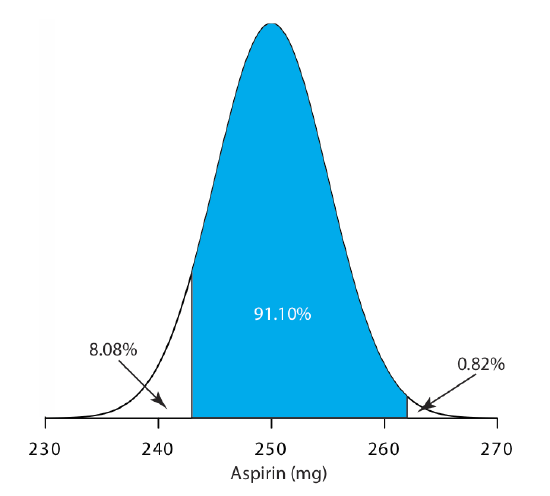
The amount of aspirin in the analgesic tablets from a particular manufacturer is known to follow a normal distribution with \(\mu\) = 250 mg and \(\sigma\) = 5. In a random sample of tablets from the production line, what percentage are expected to contain between 243 and 262 mg of aspirin?
Solution
We do not determine directly the percentage of tablets between 243 mg and 262 mg of aspirin. Instead, we first find the percentage of tablets with less than 243 mg of aspirin and the percentage of tablets having more than 262 mg of aspirin. Subtracting these results from 100%, gives the percentage of tablets that contain between 243 mg and 262 mg of aspirin.
To find the percentage of tablets with less than 243 mg of aspirin or more than 262 mg of aspirin we calculate the deviation, z, of each limit from \(\mu\) in terms of the population’s standard deviation, \(\sigma\)
\[z = \frac {X - \mu} {\sigma} \nonumber\]
where X is the limit in question. The deviation for the lower limit is
\[z_{lower} = \frac {243 - 250} {5} = -1.4 \nonumber\]
and the deviation for the upper limit is
\[z_{upper} = \frac {262 - 250} {5} = +2.4 \nonumber\]
Using the table in Appendix 3, we find that the percentage of tablets with less than 243 mg of aspirin is 8.08%, and that the percentage of tablets with more than 262 mg of aspirin is 0.82%. Therefore, the percentage of tablets containing between 243 and 262 mg of aspirin is
\[100.00 \% - 8.08 \% - 0.82 \% = 91.10 \% \nonumber\]
Figure 4.4.4 shows the distribution of aspiring in the tablets, with the area in blue showing the percentage of tablets containing between 243 mg and 262 mg of aspirin.
What percentage of aspirin tablets will contain between 240 mg and 245 mg of aspirin if the population’s mean is 250 mg and the population’s standard deviation is 5 mg.
- Answer
-
To find the percentage of tablets that contain less than 245 mg of aspirin we first calculate the deviation, z,
\[z = \frac {245 - 250} {5} = -1.00 \nonumber\]
and then look up the corresponding probability in Appendix 3, obtaining a value of 15.87%. To find the percentage of tablets that contain less than 240 mg of aspirin we find that
\[z = \frac {240 - 250} {5} = -2.00 \nonumber\]
which corresponds to 2.28%. The percentage of tablets containing between 240 and 245 mg of aspiring is 15.87% – 2.28% = 13.59%.
Confidence Intervals for Populations
If we select at random a single member from a population, what is its most likely value? This is an important question, and, in one form or another, it is at the heart of any analysis in which we wish to extrapolate from a sample to the sample’s parent population. One of the most important features of a population’s probability distribution is that it provides a way to answer this question.
Figure 4.4.3 shows that for a normal distribution, 68.26% of the population’s members have values within the range \(\mu \pm 1\sigma\). Stating this another way, there is a 68.26% probability that the result for a single sample drawn from a normally distributed population is in the interval \(\mu \pm 1\sigma\). In general, if we select a single sample we expect its value, Xi is in the range
\[X_i = \mu \pm z \sigma \label{4.2}\]
where the value of z is how confident we are in assigning this range. Values reported in this fashion are called confidence intervals. Equation \ref{4.2}, for example, is the confidence interval for a single member of a population. Table 4.4.2 gives the confidence intervals for several values of z. For reasons discussed later in the chapter, a 95% confidence level is a common choice in analytical chemistry.
When z = 1, we call this the 68.26% confidence interval.
| z | Confidence Interval |
|---|---|
| 0.50 | 38.30 |
| 1.00 | 68.26 |
| 1.50 | 86.64 |
| 1.96 | 95.00 |
| 2.00 | 95.44 |
| 2.50 | 98.76 |
| 3.00 | 99.73 |
| 3.50 | 99.95 |
What is the 95% confidence interval for the amount of aspirin in a single analgesic tablet drawn from a population for which \(\mu\) is 250 mg and for which \(\sigma\) is 5?
Solution
Using Table 4.4.2 , we find that z is 1.96 for a 95% confidence interval. Substituting this into Equation \ref{4.2} gives the confidence interval for a single tablet as
\[X_i = \mu \pm 1.96\sigma = 250 \text{ mg} \pm (1.96 \times 5) = 250 \text{ mg} \pm 10 \text{mg} \nonumber\]
A confidence interval of 250 mg ± 10 mg means that 95% of the tablets in the population contain between 240 and 260 mg of aspirin.
Alternatively, we can rewrite Equation \ref{4.2} so that it gives the confidence interval is for \(\mu\) based on the population’s standard deviation and the value of a single member drawn from the population.
\[\mu = X_i \pm z \sigma \label{4.3}\]
The population standard deviation for the amount of aspirin in a batch of analgesic tablets is known to be 7 mg of aspirin. If you randomly select and analyze a single tablet and find that it contains 245 mg of aspirin, what is the 95% confidence interval for the population’s mean?
Solution
The 95% confidence interval for the population mean is given as
\[\mu = X_i \pm z \sigma = 245 \text{ mg} \pm (1.96 \times 7) \text{ mg} = 245 \text{ mg} \pm 14 \text{ mg} \nonumber\]
Therefore, based on this one sample, we estimate that there is 95% probability that the population’s mean, \(\mu\), lies within the range of 231 mg to 259 mg of aspirin.
Note the qualification that the prediction for \(\mu\) is based on one sample; a different sample likely will give a different 95% confidence interval. Our result here, therefore, is an estimate for \(\mu\) based on this one sample.
It is unusual to predict the population’s expected mean from the analysis of a single sample; instead, we collect n samples drawn from a population of known \(\sigma\), and report the mean, X . The standard deviation of the mean, \(\sigma_{\overline{X}}\), which also is known as the standard error of the mean, is
\[\sigma_{\overline{X}} = \frac {\sigma} {\sqrt{n}} \nonumber\]
The confidence interval for the population’s mean, therefore, is
\[\mu = \overline{X} \pm \frac {z \sigma} {\sqrt{n}} \nonumber\]
What is the 95% confidence interval for the analgesic tablets in Example 4.4.4 , if an analysis of five tablets yields a mean of 245 mg of aspirin?
Solution
In this case the confidence interval is
\[\mu = 245 \text{ mg} \pm \frac {1.96 \times 7} {\sqrt{5}} \text{ mg} = 245 \text{ mg} \pm 6 \text{ mg} \nonumber\]
We estimate a 95% probability that the population’s mean is between 239 mg and 251 mg of aspirin. As expected, the confidence interval when using the mean of five samples is smaller than that for a single sample.
An analysis of seven aspirin tablets from a population known to have a standard deviation of 5, gives the following results in mg aspirin per tablet:
\(246 \quad 249 \quad 255 \quad 251 \quad 251 \quad 247 \quad 250\)
What is the 95% confidence interval for the population’s expected mean?
- Answer
-
The mean is 249.9 mg aspirin/tablet for this sample of seven tablets. For a 95% confidence interval the value of z is 1.96, which makes the confidence interval
\[249.9 \pm \frac {1.96 \times 5} {\sqrt{7}} = 249.9 \pm 3.7 \approx 250 \text{ mg} \pm 4 \text { mg} \nonumber\]
Probability Distributions for Samples
In Examples 4.4.2 –4.4.5 we assumed that the amount of aspirin in analgesic tablets is normally distributed. Without analyzing every member of the population, how can we justify this assumption? In a situation where we cannot study the whole population, or when we cannot predict the mathematical form of a population’s probability distribution, we must deduce the distribution from a limited sampling of its members.
Sample Distributions and the Central Limit Theorem
Let’s return to the problem of determining a penny’s mass to explore further the relationship between a population’s distribution and the distribution of a sample drawn from that population. The two sets of data in Table 4.4.1 are too small to provide a useful picture of a sample’s distribution, so we will use the larger sample of 100 pennies shown in Table 4.4.3 . The mean and the standard deviation for this sample are 3.095 g and 0.0346 g, respectively.
| Penny | Weight (g) | Penny | Weight (g) | Penny | Weight (g) | Penny | Weight (g) |
|---|---|---|---|---|---|---|---|
| 1 | 3.126 | 26 | 3.073 | 51 | 3.101 | 76 | 3.086 |
| 2 | 3.140 | 27 | 3.084 | 52 | 3.049 | 77 | 3.123 |
| 3 | 3.092 | 28 | 3.148 | 53 | 3.082 | 78 | 3.115 |
| 4 | 3.095 | 29 | 3.047 | 54 | 3.142 | 79 | 3.055 |
| 5 | 3.080 | 30 | 3.121 | 55 | 3.082 | 80 | 3.057 |
| 6 | 3.065 | 31 | 3.116 | 56 | 3.066 | 81 | 3.097 |
| 7 | 3.117 | 32 | 3.005 | 57 | 3.128 | 82 | 3.066 |
| 8 | 3.034 | 33 | 3.115 | 58 | 3.112 | 83 | 3.113 |
| 9 | 3.126 | 34 | 3.103 | 59 | 3.085 | 84 | 3.102 |
| 10 | 3.057 | 35 | 3.086 | 60 | 3.086 | 85 | 3.033 |
| 11 | 3.053 | 36 | 3.103 | 61 | 3.084 | 86 | 3.112 |
| 12 | 3.099 | 37 | 3.049 | 62 | 3.104 | 87 | 3.103 |
| 13 | 3.065 | 38 | 2.998 | 63 | 3.107 | 88 | 3.198 |
| 14 | 3.059 | 39 | 3.063 | 64 | 3.093 | 89 | 3.103 |
| 15 | 3.068 | 40 | 3.055 | 65 | 3.126 | 90 | 3.126 |
| 16 | 3.060 | 41 | 3.181 | 66 | 3.138 | 91 | 3.111 |
| 17 | 3.078 | 42 | 3.108 | 67 | 3.131 | 92 | 3.126 |
| 18 | 3.125 | 43 | 3.114 | 68 | 3.120 | 93 | 3.052 |
| 19 | 3.090 | 44 | 3.121 | 69 | 3.100 | 94 | 3.113 |
| 20 | 3.100 | 45 | 3.105 | 70 | 3.099 | 95 | 3.085 |
| 21 | 3.055 | 46 | 3.078 | 71 | 3.097 | 96 | 3.117 |
| 22 | 3.105 | 47 | 3.147 | 72 | 3.091 | 97 | 3.142 |
| 23 | 3.063 | 48 | 3.104 | 73 | 3.077 | 98 | 3.031 |
| 24 | 3.083 | 49 | 3.146 | 74 | 3.178 | 99 | 3.083 |
| 25 | 3.065 | 50 | 3.095 | 75 | 3.054 | 100 | 3.104 |
A histogram (Figure 4.4.5 ) is a useful way to examine the data in Table 4.4.3 . To create the histogram, we divide the sample into intervals, by mass, and determine the percentage of pennies within each interval (Table 4.4.4 ). Note that the sample’s mean is the midpoint of the histogram.
| Mass Interval | Frequency (as % of Sample) | Mass Interval | Frequency (as % of Sample) |
|---|---|---|---|
| 2.991 – 3.009 | 2 | 3.105 – 3.123 | 19 |
| 3.010 – 3.028 | 0 | 3.124 – 3.142 | 12 |
| 3.029 – 3.047 | 4 | 3.143 – 3.161 | 3 |
| 3.048 – 3.066 | 19 | 3.162 – 3.180 | 1 |
| 3.067 – 3.085 | 14 | 3.181 – 3.199 | 2 |
| 3.086 – 3.104 | 24 | 3.200 – 3.218 | 0 |
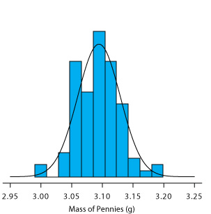
Figure 4.4.5 also includes a normal distribution curve for the population of pennies, based on the assumption that the mean and the variance for the sample are appropriate estimates for the population’s mean and variance. Although the histogram is not perfectly symmetric in shape, it provides a good approximation of the normal distribution curve, suggesting that the sample of 100 pennies is normally distributed. It is easy to imagine that the histogram will approximate more closely a normal distribution if we include additional pennies in our sample.
We will not offer a formal proof that the sample of pennies in Table 4.4.3 and the population of all circulating U. S. pennies are normally distributed; however, the evidence in Figure 4.4.5 strongly suggests this is true. Although we cannot claim that the results of all experiments are normally distributed, in most cases our data are normally distributed. According to the central limit theorem, when a measurement is subject to a variety of indeterminate errors, the results for that measurement will approximate a normal distribution [Mark, H.; Workman, J. Spectroscopy 1988, 3, 44–48]. The central limit theorem holds true even if the individual sources of indeterminate error are not normally distributed. The chief limitation to the central limit theorem is that the sources of indeterminate error must be independent and of similar magnitude so that no one source of error dominates the final distribution.
An additional feature of the central limit theorem is that a distribution of means for samples drawn from a population with any distribution will approximate closely a normal distribution if the size of each sample is sufficiently large. For example, Figure 4.4.6 shows the distribution for two samples of 10 000 drawn from a uniform distribution in which every value between 0 and 1 occurs with an equal frequency. For samples of size n = 1, the resulting distribution closely approximates the population’s uniform distribution. The distribution of the means for samples of size n = 10, however, closely approximates a normal distribution.
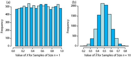
You might reasonably ask whether this aspect of the central limit theorem is important as it is unlikely that we will complete 10 000 analyses, each of which is the average of 10 individual trials. This is deceiving. When we acquire a sample of soil, for example, it consists of many individual particles each of which is an individual sample of the soil. Our analysis of this sample, therefore, gives the mean for this large number of individual soil particles. Because of this, the central limit theorem is relevant. For a discussion of circumstances where the central limit theorem may not apply, see “Do You Reckon It’s Normally Distributed?”, the full reference for which is Majewsky, M.; Wagner, M.; Farlin, J. Sci. Total Environ. 2016, 548–549, 408–409.
Degrees of Freedom
Did you notice the differences between the equation for the variance of a population and the variance of a sample? If not, here are the two equations:
\[\sigma^2 = \frac {\sum_{i = 1}^n (X_i - \mu)^2} {n} \nonumber\]
\[s^2 = \frac {\sum_{i = 1}^n (X_i - \overline{X})^2} {n - 1} \nonumber\]
Both equations measure the variance around the mean, using \(\mu\) for a population and \(\overline{X}\) for a sample. Although the equations use different measures for the mean, the intention is the same for both the sample and the population. A more interesting difference is between the denominators of the two equations. When we calculate the population’s variance we divide the numerator by the population’s size, n; for the sample’s variance, however, we divide by n – 1, where n is the sample’s size. Why do we divide by n – 1 when we calculate the sample’s variance?
A variance is the average squared deviation of individual results relative to the mean. When we calculate an average we divide the sum by the number of independent measurements, or degrees of freedom, in the calculation. For the population’s variance, the degrees of freedom is equal to the population’s size, n. When we measure every member of a population we have complete information about the population.
When we calculate the sample’s variance, however, we replace \(\mu\) with \(\overline{X}\), which we also calculate using the same data. If there are n members in the sample, we can deduce the value of the nth member from the remaining n – 1 members and the mean. For example, if \(n = 5\) and we know that the first four samples are 1, 2, 3 and 4, and that the mean is 3, then the fifth member of the sample must be
\[X_5 = (\overline{X} \times n) - X_1 - X_2 - X_3 - X_4 = (3 \times 5) - 1 - 2 - 3 - 4 = 5 \nonumber\]
Because we have just four independent measurements, we have lost one degree of freedom. Using n – 1 in place of n when we calculate the sample’s variance ensures that \(s^2\) is an unbiased estimator of \(\sigma^2\).
Here is another way to think about degrees of freedom. We analyze samples to make predictions about the underlying population. When our sample consists of n measurements we cannot make more than n independent predictions about the population. Each time we estimate a parameter, such as the population’s mean, we lose a degree of freedom. If there are n degrees of freedom for calculating the sample’s mean, then n – 1 degrees of freedom remain when we calculate the sample’s variance.
Confidence Intervals for Samples
Earlier we introduced the confidence interval as a way to report the most probable value for a population’s mean, \(\mu\)
\[\mu = \overline{X} \pm \frac {z \sigma} {\sqrt{n}} \label{4.4}\]
where \(\overline{X}\) is the mean for a sample of size n, and \(\sigma\) is the population’s standard deviation. For most analyses we do not know the population’s standard deviation. We can still calculate a confidence interval, however, if we make two modifications to Equation \ref{4.4}.
The first modification is straightforward—we replace the population’s standard deviation, \(\sigma\), with the sample’s standard deviation, s. The second modification is not as obvious. The values of z in Table 4.4.2 are for a normal distribution, which is a function of \(sigma^2\), not s2. Although the sample’s variance, s2, is an unbiased estimate of the population’s variance, \(\sigma^2\), the value of s2 will only rarely equal \(\sigma^2\). To account for this uncertainty in estimating \(\sigma^2\), we replace the variable z in Equation \ref{4.4} with the variable t, where t is defined such that \(t \ge z\) at all confidence levels.
\[\mu = \overline{X} \pm \frac {t s} {\sqrt{n}} \label{4.5}\]
Values for t at the 95% confidence level are shown in Table 4.4.5 . Note that t becomes smaller as the number of degrees of freedom increases, and that it approaches z as n approaches infinity. The larger the sample, the more closely its confidence interval for a sample (Equation \ref{4.5}) approaches the confidence interval for the population (Equation \ref{4.3}). Appendix 4 provides additional values of t for other confidence levels.
| Degrees of Freedom | t | Degrees of Freedom | t | Degrees of Freedom | t | Degrees of Freedom | t |
|---|---|---|---|---|---|---|---|
| 1 | 12.706 | 6 | 2.447 | 12 | 2.179 | 30 | 2.042 |
| 2 | 4.303 | 7 | 2.365 | 14 | 2.145 | 40 | 2.021 |
| 3 | 3.181 | 8 | 2.306 | 16 | 2.120 | 60 | 2.000 |
| 4 | 2.776 | 9 | 2.262 | 18 | 2.101 | 100 | 1.984 |
| 5 | 2.571 | 10 | 2.228 | 20 | 2.086 | \(\infty | 1.960 |
What are the 95% confidence intervals for the two samples of pennies in Table 4.4.1 ?
Solution
The mean and the standard deviation for first experiment are, respectively, 3.117 g and 0.051 g. Because the sample consists of seven measurements, there are six degrees of freedom. The value of t from Table 4.4.5 , is 2.447. Substituting into Equation \ref{4.5} gives
\[\mu = 3.117 \text{ g} \pm \frac {2.447 \times 0.051 \text{ g}} {\sqrt{7}} = 3.117 \text{ g} \pm 0.047 \text{ g} \nonumber\]
For the second experiment the mean and the standard deviation are 3.081 g and 0.073 g, respectively, with four degrees of freedom. The 95% confidence interval is
\[\mu = 3.081 \text{ g} \pm \frac {2.776 \times 0.037 \text{ g}} {\sqrt{5}} = 3.081 \text{ g} \pm 0.046 \text{ g} \nonumber\]
Based on the first experiment, the 95% confidence interval for the population’s mean is 3.070–3.164 g. For the second experiment, the 95% confidence interval is 3.035–3.127 g. Although the two confidence intervals are not identical—remember, each confidence interval provides a different estimate for \(\mu\)—the mean for each experiment is contained within the other experiment’s confidence interval. There also is an appreciable overlap of the two confidence intervals. Both of these observations are consistent with samples drawn from the same population.
Note that our comparison of these two confidence intervals at this point is somewhat vague and unsatisfying. We will return to this point in the next section, when we consider a statistical approach to comparing the results of experiments.
What is the 95% confidence interval for the sample of 100 pennies in Table 4.4.3 ? The mean and the standard deviation for this sample are 3.095 g and 0.0346 g, respectively. Compare your result to the confidence intervals for the samples of pennies in Table 4.4.1 .
- Answer
-
With 100 pennies, we have 99 degrees of freedom for the mean. Although Table 4.4.3 does not include a value for t(0.05, 99), we can approximate its value by using the values for t(0.05, 60) and t(0.05, 100) and by assuming a linear change in its value.
\[t(0.05, 99) = t(0.05, 60) - \frac {39} {40} \left\{ t(0.05, 60) - t(0.05, 100\} \right) \nonumber\]
\[t(0.05, 99) = 2.000 - \frac {39} {40} \left\{ 2.000 - 1.984 \right\} = 1.9844 \nonumber\]
The 95% confidence interval for the pennies is
\[3.095 \pm \frac {1.9844 \times 0.0346} {\sqrt{100}} = 3.095 \text{ g} \pm 0.007 \text{ g} \nonumber\]
From Example 4.4.6 , the 95% confidence intervals for the two samples in Table 4.4.1 are 3.117 g ± 0.047 g and 3.081 g ± 0.046 g. As expected, the confidence interval for the sample of 100 pennies is much smaller than that for the two smaller samples of pennies. Note, as well, that the confidence interval for the larger sample fits within the confidence intervals for the two smaller samples.
A Cautionary Statement
There is a temptation when we analyze data simply to plug numbers into an equation, carry out the calculation, and report the result. This is never a good idea, and you should develop the habit of reviewing and evaluating your data. For example, if you analyze five samples and report an analyte’s mean concentration as 0.67 ppm with a standard deviation of 0.64 ppm, then the 95% confidence interval is
\[\mu = 0.67 \text{ ppm} \pm \frac {2.776 \times 0.64 \text{ ppm}} {\sqrt{5}} = 0.67 \text{ ppm} \pm 0.79 \text{ ppm} \nonumber\]
This confidence interval estimates that the analyte’s true concentration is between –0.12 ppm and 1.46 ppm. Including a negative concentration within the confidence interval should lead you to reevaluate your data or your conclusions. A closer examination of your data may convince you that the standard deviation is larger than expected, making the confidence interval too broad, or you may conclude that the analyte’s concentration is too small to report with confidence.
We will return to the topic of detection limits near the end of this chapter.
Here is a second example of why you should closely examine your data: results obtained on samples drawn at random from a normally distributed population must be random. If the results for a sequence of samples show a regular pattern or trend, then the underlying population either is not normally distributed or there is a time-dependent determinate error. For example, if we randomly select 20 pennies and find that the mass of each penny is greater than that for the preceding penny, then we might suspect that our balance is drifting out of calibration.