Search

Text Color

Margin Size

Font Type

Enable Dyslexic Font

Recovery Curves and Signal Averaging

Last updated

Oct 20, 2020
Save as PDF
- Quantitative Fluorescence
- Redox Reactions

Contributor
Analytical Sciences Digital Library

$\newcommand{\vecs}[1]{\overset { \scriptstyle \rightharpoonup} {\mathbf{#1}} }$

$\newcommand{\vecd}[1]{\overset{-\!-\!\rightharpoonup}{\vphantom{a}\smash {#1}}}$

$\newcommand{\id}{\mathrm{id}}$ $\newcommand{\Span}{\mathrm{span}}$

( \newcommand{\kernel}{\mathrm{null}\,}\) $\newcommand{\range}{\mathrm{range}\,}$

$\newcommand{\RealPart}{\mathrm{Re}}$ $\newcommand{\ImaginaryPart}{\mathrm{Im}}$

$\newcommand{\Argument}{\mathrm{Arg}}$ $\newcommand{\norm}[1]{\| #1 \|}$

$\newcommand{\inner}[2]{\langle #1, #2 \rangle}$

$\newcommand{\Span}{\mathrm{span}}$

$\newcommand{\id}{\mathrm{id}}$

$\newcommand{\Span}{\mathrm{span}}$

$\newcommand{\kernel}{\mathrm{null}\,}$

$\newcommand{\range}{\mathrm{range}\,}$

$\newcommand{\RealPart}{\mathrm{Re}}$

$\newcommand{\ImaginaryPart}{\mathrm{Im}}$

$\newcommand{\Argument}{\mathrm{Arg}}$

$\newcommand{\norm}[1]{\| #1 \|}$

$\newcommand{\inner}[2]{\langle #1, #2 \rangle}$

$\newcommand{\Span}{\mathrm{span}}$ $\newcommand{\AA}{\unicode[.8,0]{x212B}}$

$\newcommand{\vectorA}[1]{\vec{#1}} % arrow$

$\newcommand{\vectorAt}[1]{\vec{\text{#1}}} % arrow$

$\newcommand{\vectorB}[1]{\overset { \scriptstyle \rightharpoonup} {\mathbf{#1}} }$

$\newcommand{\vectorC}[1]{\textbf{#1}}$

$\newcommand{\vectorD}[1]{\overrightarrow{#1}}$

$\newcommand{\vectorDt}[1]{\overrightarrow{\text{#1}}}$

$\newcommand{\vectE}[1]{\overset{-\!-\!\rightharpoonup}{\vphantom{a}\smash{\mathbf {#1}}}}$

$\newcommand{\vecs}[1]{\overset { \scriptstyle \rightharpoonup} {\mathbf{#1}} }$

$\newcommand{\vecd}[1]{\overset{-\!-\!\rightharpoonup}{\vphantom{a}\smash {#1}}}$

$\newcommand{\avec}{\mathbf a}$

$\newcommand{\bvec}{\mathbf b}$

$\newcommand{\cvec}{\mathbf c}$

$\newcommand{\dvec}{\mathbf d}$

$\newcommand{\dtil}{\widetilde{\mathbf d}}$

$\newcommand{\evec}{\mathbf e}$

$\newcommand{\fvec}{\mathbf f}$

$\newcommand{\nvec}{\mathbf n}$

$\newcommand{\pvec}{\mathbf p}$

$\newcommand{\qvec}{\mathbf q}$

$\newcommand{\svec}{\mathbf s}$

$\newcommand{\tvec}{\mathbf t}$

$\newcommand{\uvec}{\mathbf u}$

$\newcommand{\vvec}{\mathbf v}$

$\newcommand{\wvec}{\mathbf w}$

$\newcommand{\xvec}{\mathbf x}$

$\newcommand{\yvec}{\mathbf y}$

$\newcommand{\zvec}{\mathbf z}$

$\newcommand{\rvec}{\mathbf r}$

$\newcommand{\mvec}{\mathbf m}$

$\newcommand{\zerovec}{\mathbf 0}$

$\newcommand{\onevec}{\mathbf 1}$

$\newcommand{\real}{\mathbb R}$

$\newcommand{\twovec}[2]{\left[\begin{array}{r}#1 \\ #2 \end{array}\right]}$

$\newcommand{\ctwovec}[2]{\left[\begin{array}{c}#1 \\ #2 \end{array}\right]}$

$\newcommand{\threevec}[3]{\left[\begin{array}{r}#1 \\ #2 \\ #3 \end{array}\right]}$

$\newcommand{\cthreevec}[3]{\left[\begin{array}{c}#1 \\ #2 \\ #3 \end{array}\right]}$

$\newcommand{\fourvec}[4]{\left[\begin{array}{r}#1 \\ #2 \\ #3 \\ #4 \end{array}\right]}$

$\newcommand{\cfourvec}[4]{\left[\begin{array}{c}#1 \\ #2 \\ #3 \\ #4 \end{array}\right]}$

$\newcommand{\fivevec}[5]{\left[\begin{array}{r}#1 \\ #2 \\ #3 \\ #4 \\ #5 \\ \end{array}\right]}$

$\newcommand{\cfivevec}[5]{\left[\begin{array}{c}#1 \\ #2 \\ #3 \\ #4 \\ #5 \\ \end{array}\right]}$

$\newcommand{\mattwo}[4]{\left[\begin{array}{rr}#1 \amp #2 \\ #3 \amp #4 \\ \end{array}\right]}$

$\newcommand{\laspan}[1]{\text{Span}\{#1\}}$

$\newcommand{\bcal}{\cal B}$

$\newcommand{\ccal}{\cal C}$

$\newcommand{\scal}{\cal S}$

$\newcommand{\wcal}{\cal W}$

$\newcommand{\ecal}{\cal E}$

$\newcommand{\coords}[2]{\left\{#1\right\}_{#2}}$

$\newcommand{\gray}[1]{\color{gray}{#1}}$

$\newcommand{\lgray}[1]{\color{lightgray}{#1}}$

$\newcommand{\rank}{\operatorname{rank}}$

$\newcommand{\row}{\text{Row}}$

$\newcommand{\col}{\text{Col}}$

$\renewcommand{\row}{\text{Row}}$

$\newcommand{\nul}{\text{Nul}}$

$\newcommand{\var}{\text{Var}}$

$\newcommand{\corr}{\text{corr}}$

$\newcommand{\len}[1]{\left|#1\right|}$

$\newcommand{\bbar}{\overline{\bvec}}$

$\newcommand{\bhat}{\widehat{\bvec}}$

$\newcommand{\bperp}{\bvec^\perp}$

$\newcommand{\xhat}{\widehat{\xvec}}$

$\newcommand{\vhat}{\widehat{\vvec}}$

$\newcommand{\uhat}{\widehat{\uvec}}$

$\newcommand{\what}{\widehat{\wvec}}$

$\newcommand{\Sighat}{\widehat{\Sigma}}$

$\newcommand{\lt}{<}$

$\newcommand{\gt}{>}$

$\newcommand{\amp}{&}$

$\definecolor{fillinmathshade}{gray}{0.9}$

Classroom Exercise #4: Recovery Curves and Signal Averaging

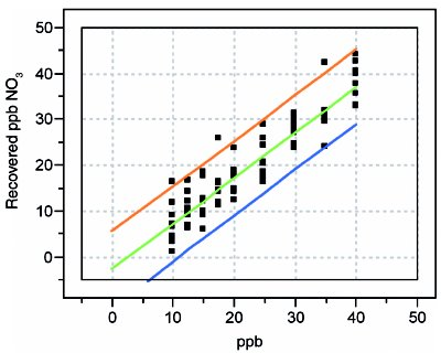
The following are recovery plots of anion analysis from soil. The graphs plot recovered anion in ppb vs the amount that was spiked in. The anion measured for each is in the y-axis label.

The center line is the average, while the outer 2 lines are the 95 % confidence interval.

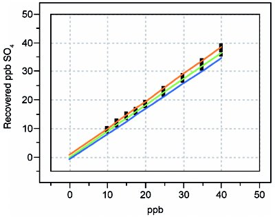
A. Look at the axis of the graphs. What is the ideal slope of these plots? Which plot is most ideal (F, SO₄, NO₃) and why?
1. What is the problem in the F plot? What error could account for that problem?
2. What is the problem in the NO₃ plot? What error could account for that problem?
3. Why is important to know the confidence limit as well as the average for these plots?

Moving average. Sheet 1 of the Excel spreadsheet has a chromatogram.
First plot the data (first column is time in min, second signal in arbitrary absorbance units). Then find an area of flat baseline. Use the data in that place to calculate the noise (i.e. standard deviation).

What is the noise? ____________

What is the maximum peak height? ____________

What is the S/N? _____________

Next, use Excel’s average function to make a 5 point moving average smoothed chromatogram. The first 2 points are hard (you can leave them as is), but after that average the two points before a point, that point and the two points after the point. Plot this data. Use the same area of flat baseline and calculate the noise.

What is the noise? ____________

What is the maximum peak height? ____________

What is the S/N? _____________________

What do you notice about the smoothed chromatogram, in terms of signal, noise, or other features?

Signal Averaging
Sheet 2 of the Excel Sheet has example data for signal averaging. In this case, a short chromatogram is given, first as ideal noiseless data, then with noise added (I used a random number generator to add the same amount of noise in this case for each trial).

Plot the noiseless data vs. time.

Now plot all the trials on one graph.

Find a portion of the baseline to use to calculate noise, in Excel, calculate the standard deviation of this portion of the baseline for each trial. What is the average of those standard deviations? ____________

Now average the 9 trials together (do not include the noiseless data).

Calculate the noise of the same part of the baseline: _________

How much does the noise differ by? _________

What factor would you have predicted, given we did 9 replicates? ___________

Plot the averaged data on its own graph. Is it easier to see the peaks? For which peak does it matter most?

Excel Syntax

AVERAGE(number1, [number2], ...)

STDEV.S(number1,[number2],...) Gives the sample standard deviation

STDEV.P(number1,[number2],...) Gives the population standard deviation

Contributors and Attributions

Jill Venton, University of Virginia (bjv2n@eservices.virginia.edu)
Sourced from the Analytical Sciences Digital Library

Contributors and Attributions

Support Center

How can we help?