5.1: Basic Principles
- Page ID
- 212585
\( \newcommand{\vecs}[1]{\overset { \scriptstyle \rightharpoonup} {\mathbf{#1}} } \)
\( \newcommand{\vecd}[1]{\overset{-\!-\!\rightharpoonup}{\vphantom{a}\smash {#1}}} \)
\( \newcommand{\dsum}{\displaystyle\sum\limits} \)
\( \newcommand{\dint}{\displaystyle\int\limits} \)
\( \newcommand{\dlim}{\displaystyle\lim\limits} \)
\( \newcommand{\id}{\mathrm{id}}\) \( \newcommand{\Span}{\mathrm{span}}\)
( \newcommand{\kernel}{\mathrm{null}\,}\) \( \newcommand{\range}{\mathrm{range}\,}\)
\( \newcommand{\RealPart}{\mathrm{Re}}\) \( \newcommand{\ImaginaryPart}{\mathrm{Im}}\)
\( \newcommand{\Argument}{\mathrm{Arg}}\) \( \newcommand{\norm}[1]{\| #1 \|}\)
\( \newcommand{\inner}[2]{\langle #1, #2 \rangle}\)
\( \newcommand{\Span}{\mathrm{span}}\)
\( \newcommand{\id}{\mathrm{id}}\)
\( \newcommand{\Span}{\mathrm{span}}\)
\( \newcommand{\kernel}{\mathrm{null}\,}\)
\( \newcommand{\range}{\mathrm{range}\,}\)
\( \newcommand{\RealPart}{\mathrm{Re}}\)
\( \newcommand{\ImaginaryPart}{\mathrm{Im}}\)
\( \newcommand{\Argument}{\mathrm{Arg}}\)
\( \newcommand{\norm}[1]{\| #1 \|}\)
\( \newcommand{\inner}[2]{\langle #1, #2 \rangle}\)
\( \newcommand{\Span}{\mathrm{span}}\) \( \newcommand{\AA}{\unicode[.8,0]{x212B}}\)
\( \newcommand{\vectorA}[1]{\vec{#1}} % arrow\)
\( \newcommand{\vectorAt}[1]{\vec{\text{#1}}} % arrow\)
\( \newcommand{\vectorB}[1]{\overset { \scriptstyle \rightharpoonup} {\mathbf{#1}} } \)
\( \newcommand{\vectorC}[1]{\textbf{#1}} \)
\( \newcommand{\vectorD}[1]{\overrightarrow{#1}} \)
\( \newcommand{\vectorDt}[1]{\overrightarrow{\text{#1}}} \)
\( \newcommand{\vectE}[1]{\overset{-\!-\!\rightharpoonup}{\vphantom{a}\smash{\mathbf {#1}}}} \)
\( \newcommand{\vecs}[1]{\overset { \scriptstyle \rightharpoonup} {\mathbf{#1}} } \)
\(\newcommand{\longvect}{\overrightarrow}\)
\( \newcommand{\vecd}[1]{\overset{-\!-\!\rightharpoonup}{\vphantom{a}\smash {#1}}} \)
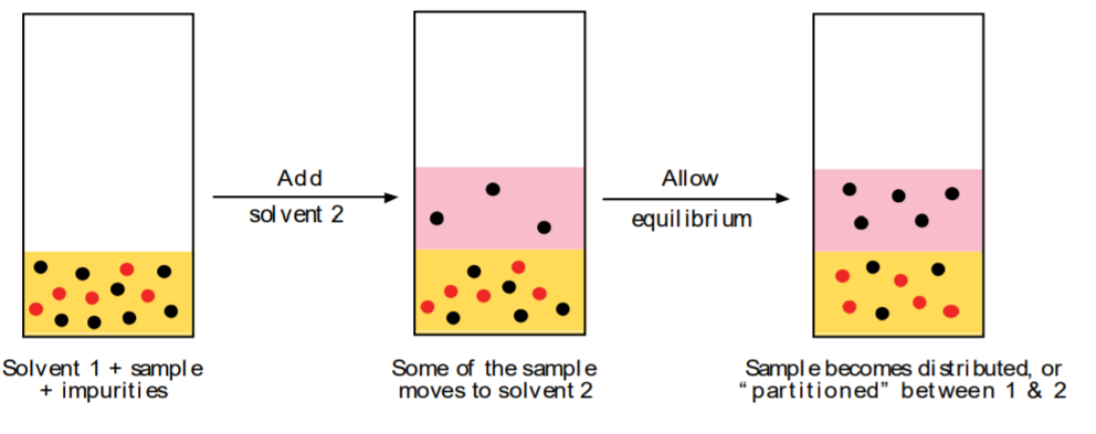
\(\newcommand{\avec}{\mathbf a}\) \(\newcommand{\bvec}{\mathbf b}\) \(\newcommand{\cvec}{\mathbf c}\) \(\newcommand{\dvec}{\mathbf d}\) \(\newcommand{\dtil}{\widetilde{\mathbf d}}\) \(\newcommand{\evec}{\mathbf e}\) \(\newcommand{\fvec}{\mathbf f}\) \(\newcommand{\nvec}{\mathbf n}\) \(\newcommand{\pvec}{\mathbf p}\) \(\newcommand{\qvec}{\mathbf q}\) \(\newcommand{\svec}{\mathbf s}\) \(\newcommand{\tvec}{\mathbf t}\) \(\newcommand{\uvec}{\mathbf u}\) \(\newcommand{\vvec}{\mathbf v}\) \(\newcommand{\wvec}{\mathbf w}\) \(\newcommand{\xvec}{\mathbf x}\) \(\newcommand{\yvec}{\mathbf y}\) \(\newcommand{\zvec}{\mathbf z}\) \(\newcommand{\rvec}{\mathbf r}\) \(\newcommand{\mvec}{\mathbf m}\) \(\newcommand{\zerovec}{\mathbf 0}\) \(\newcommand{\onevec}{\mathbf 1}\) \(\newcommand{\real}{\mathbb R}\) \(\newcommand{\twovec}[2]{\left[\begin{array}{r}#1 \\ #2 \end{array}\right]}\) \(\newcommand{\ctwovec}[2]{\left[\begin{array}{c}#1 \\ #2 \end{array}\right]}\) \(\newcommand{\threevec}[3]{\left[\begin{array}{r}#1 \\ #2 \\ #3 \end{array}\right]}\) \(\newcommand{\cthreevec}[3]{\left[\begin{array}{c}#1 \\ #2 \\ #3 \end{array}\right]}\) \(\newcommand{\fourvec}[4]{\left[\begin{array}{r}#1 \\ #2 \\ #3 \\ #4 \end{array}\right]}\) \(\newcommand{\cfourvec}[4]{\left[\begin{array}{c}#1 \\ #2 \\ #3 \\ #4 \end{array}\right]}\) \(\newcommand{\fivevec}[5]{\left[\begin{array}{r}#1 \\ #2 \\ #3 \\ #4 \\ #5 \\ \end{array}\right]}\) \(\newcommand{\cfivevec}[5]{\left[\begin{array}{c}#1 \\ #2 \\ #3 \\ #4 \\ #5 \\ \end{array}\right]}\) \(\newcommand{\mattwo}[4]{\left[\begin{array}{rr}#1 \amp #2 \\ #3 \amp #4 \\ \end{array}\right]}\) \(\newcommand{\laspan}[1]{\text{Span}\{#1\}}\) \(\newcommand{\bcal}{\cal B}\) \(\newcommand{\ccal}{\cal C}\) \(\newcommand{\scal}{\cal S}\) \(\newcommand{\wcal}{\cal W}\) \(\newcommand{\ecal}{\cal E}\) \(\newcommand{\coords}[2]{\left\{#1\right\}_{#2}}\) \(\newcommand{\gray}[1]{\color{gray}{#1}}\) \(\newcommand{\lgray}[1]{\color{lightgray}{#1}}\) \(\newcommand{\rank}{\operatorname{rank}}\) \(\newcommand{\row}{\text{Row}}\) \(\newcommand{\col}{\text{Col}}\) \(\renewcommand{\row}{\text{Row}}\) \(\newcommand{\nul}{\text{Nul}}\) \(\newcommand{\var}{\text{Var}}\) \(\newcommand{\corr}{\text{corr}}\) \(\newcommand{\len}[1]{\left|#1\right|}\) \(\newcommand{\bbar}{\overline{\bvec}}\) \(\newcommand{\bhat}{\widehat{\bvec}}\) \(\newcommand{\bperp}{\bvec^\perp}\) \(\newcommand{\xhat}{\widehat{\xvec}}\) \(\newcommand{\vhat}{\widehat{\vvec}}\) \(\newcommand{\uhat}{\widehat{\uvec}}\) \(\newcommand{\what}{\widehat{\wvec}}\) \(\newcommand{\Sighat}{\widehat{\Sigma}}\) \(\newcommand{\lt}{<}\) \(\newcommand{\gt}{>}\) \(\newcommand{\amp}{&}\) \(\definecolor{fillinmathshade}{gray}{0.9}\)The technique of liquid-liquid extraction is used to purify impure substances by taking advantage of a solubility differential of the substance in different solvents. It is different from crystallization in that the sample can be solid or liquid. The impure sample is dissolved in solvent 1 first. Then a second solvent 2 is added in such a way that the sample migrates from the first to the second solvent without the impurities. This, of course, requires that the two solvents 1 and 2 be immiscible, and ideally that the sample be more soluble in solvent 2 than in solvent 1.

The process described above is called extraction, and solvent 2 is referred to as the extracting solvent. Since the sample is soluble in both solvents, it will “partition,” or become distributed, between the two. The final ratio of the concentrations of the sample in the two solvents is determined by its distribution (or partition) coefficient K.
In microscale it is convenient to express the concentration in mg of solute/mL of solution. After extraction, the final, or equilibrium, concentration of the sample in the original solvent (1) is given by C1, and the concentration of sample in the extracting solvent (2) is given by C2. The distribution coefficient is defined as the ratio of the two concentrations, with C2 as the numerator.
\(K = \frac{C_{2}}{C_{1}}\)
Needless to say, the greater the concentration of sample in the extracting solvent, the greater the distribution coefficient, and the more efficient the extraction.
EXAMPLE: Calculating the amount of extracted solute in a single extraction, knowing K. Refer to fig. 12.2, p. 672 in your lab textbook. As a point of departure, we have a solution of 50 mg sample in 1 mL aqueous solution. We extract once by adding 0.5 mL ether. After shaking, an unknown amount of solute (x mg) will remain in solvent 1 (water), and the rest (50-x mg) will migrate to solvent 2 (ether). Therefore the equilibrium (or final) concentrations of solute in the two solvents are:
\(C_{1} = \frac{x mg}{1mL} =x \frac{mg}{mL}\)
and \(C_{2} = \frac{(50-x)mg}{0.5 mL} = 2(50-x) \frac{mg}{mL} = (100-2x) \frac{mg}{mL}\)
\(C_{2} = \frac{(50-x)mg}{0.5mL} = 2(50-x) \frac{mg}{mL} = (100-2x) \frac{mg}{mL}\)
The distribution coefficient K must be given in order to do the calculations. In this case it has a value of 10. Therefore:
\(K = 100 = \frac{(100-2x)}{x}\)
\(100 - 2x = 10x\)
\(100 = 10x + 2x = 12x
\(x = \frac{100}{12} = 8.3mg\) solute remain in the water
\(50-x = 50 - 8.3 = 41.7mg\) sample have moved to the ether (83.4% or original amount)
Make sure to review the calculations shown on p. 671. These are intended to demonstrate that it is more effective to extract more times with smaller amounts of extracting solvent than fewer times with larger amounts of extracting solvent. Then go back and compare fig. 12.2 and 12.3 (p. 672-673) for a visual illustration of the same principle.
To test your understanding of these concepts, do the prelab calculation at the top of p. 34.
The following practical observations apply when performing extractions in the lab:
1. Performing two or three extractions gets most of the sample out of the original solvent, provided that is favorable (at least 5 or greater) K .
2. The more concentrated the solutions, the more efficient the extraction. That’s another reason for using small amounts of solvent during extractions.
3. If the original solution is too dilute, it’s better to increase its concentration before the extraction by evaporating some of the solvent.


