3: ab initio Calculations - Dihydrogen Potential Curve (Dry Lab)
- Page ID
- 65237
\( \newcommand{\vecs}[1]{\overset { \scriptstyle \rightharpoonup} {\mathbf{#1}} } \)
\( \newcommand{\vecd}[1]{\overset{-\!-\!\rightharpoonup}{\vphantom{a}\smash {#1}}} \)
\( \newcommand{\dsum}{\displaystyle\sum\limits} \)
\( \newcommand{\dint}{\displaystyle\int\limits} \)
\( \newcommand{\dlim}{\displaystyle\lim\limits} \)
\( \newcommand{\id}{\mathrm{id}}\) \( \newcommand{\Span}{\mathrm{span}}\)
( \newcommand{\kernel}{\mathrm{null}\,}\) \( \newcommand{\range}{\mathrm{range}\,}\)
\( \newcommand{\RealPart}{\mathrm{Re}}\) \( \newcommand{\ImaginaryPart}{\mathrm{Im}}\)
\( \newcommand{\Argument}{\mathrm{Arg}}\) \( \newcommand{\norm}[1]{\| #1 \|}\)
\( \newcommand{\inner}[2]{\langle #1, #2 \rangle}\)
\( \newcommand{\Span}{\mathrm{span}}\)
\( \newcommand{\id}{\mathrm{id}}\)
\( \newcommand{\Span}{\mathrm{span}}\)
\( \newcommand{\kernel}{\mathrm{null}\,}\)
\( \newcommand{\range}{\mathrm{range}\,}\)
\( \newcommand{\RealPart}{\mathrm{Re}}\)
\( \newcommand{\ImaginaryPart}{\mathrm{Im}}\)
\( \newcommand{\Argument}{\mathrm{Arg}}\)
\( \newcommand{\norm}[1]{\| #1 \|}\)
\( \newcommand{\inner}[2]{\langle #1, #2 \rangle}\)
\( \newcommand{\Span}{\mathrm{span}}\) \( \newcommand{\AA}{\unicode[.8,0]{x212B}}\)
\( \newcommand{\vectorA}[1]{\vec{#1}} % arrow\)
\( \newcommand{\vectorAt}[1]{\vec{\text{#1}}} % arrow\)
\( \newcommand{\vectorB}[1]{\overset { \scriptstyle \rightharpoonup} {\mathbf{#1}} } \)
\( \newcommand{\vectorC}[1]{\textbf{#1}} \)
\( \newcommand{\vectorD}[1]{\overrightarrow{#1}} \)
\( \newcommand{\vectorDt}[1]{\overrightarrow{\text{#1}}} \)
\( \newcommand{\vectE}[1]{\overset{-\!-\!\rightharpoonup}{\vphantom{a}\smash{\mathbf {#1}}}} \)
\( \newcommand{\vecs}[1]{\overset { \scriptstyle \rightharpoonup} {\mathbf{#1}} } \)
\(\newcommand{\longvect}{\overrightarrow}\)
\( \newcommand{\vecd}[1]{\overset{-\!-\!\rightharpoonup}{\vphantom{a}\smash {#1}}} \)
\(\newcommand{\avec}{\mathbf a}\) \(\newcommand{\bvec}{\mathbf b}\) \(\newcommand{\cvec}{\mathbf c}\) \(\newcommand{\dvec}{\mathbf d}\) \(\newcommand{\dtil}{\widetilde{\mathbf d}}\) \(\newcommand{\evec}{\mathbf e}\) \(\newcommand{\fvec}{\mathbf f}\) \(\newcommand{\nvec}{\mathbf n}\) \(\newcommand{\pvec}{\mathbf p}\) \(\newcommand{\qvec}{\mathbf q}\) \(\newcommand{\svec}{\mathbf s}\) \(\newcommand{\tvec}{\mathbf t}\) \(\newcommand{\uvec}{\mathbf u}\) \(\newcommand{\vvec}{\mathbf v}\) \(\newcommand{\wvec}{\mathbf w}\) \(\newcommand{\xvec}{\mathbf x}\) \(\newcommand{\yvec}{\mathbf y}\) \(\newcommand{\zvec}{\mathbf z}\) \(\newcommand{\rvec}{\mathbf r}\) \(\newcommand{\mvec}{\mathbf m}\) \(\newcommand{\zerovec}{\mathbf 0}\) \(\newcommand{\onevec}{\mathbf 1}\) \(\newcommand{\real}{\mathbb R}\) \(\newcommand{\twovec}[2]{\left[\begin{array}{r}#1 \\ #2 \end{array}\right]}\) \(\newcommand{\ctwovec}[2]{\left[\begin{array}{c}#1 \\ #2 \end{array}\right]}\) \(\newcommand{\threevec}[3]{\left[\begin{array}{r}#1 \\ #2 \\ #3 \end{array}\right]}\) \(\newcommand{\cthreevec}[3]{\left[\begin{array}{c}#1 \\ #2 \\ #3 \end{array}\right]}\) \(\newcommand{\fourvec}[4]{\left[\begin{array}{r}#1 \\ #2 \\ #3 \\ #4 \end{array}\right]}\) \(\newcommand{\cfourvec}[4]{\left[\begin{array}{c}#1 \\ #2 \\ #3 \\ #4 \end{array}\right]}\) \(\newcommand{\fivevec}[5]{\left[\begin{array}{r}#1 \\ #2 \\ #3 \\ #4 \\ #5 \\ \end{array}\right]}\) \(\newcommand{\cfivevec}[5]{\left[\begin{array}{c}#1 \\ #2 \\ #3 \\ #4 \\ #5 \\ \end{array}\right]}\) \(\newcommand{\mattwo}[4]{\left[\begin{array}{rr}#1 \amp #2 \\ #3 \amp #4 \\ \end{array}\right]}\) \(\newcommand{\laspan}[1]{\text{Span}\{#1\}}\) \(\newcommand{\bcal}{\cal B}\) \(\newcommand{\ccal}{\cal C}\) \(\newcommand{\scal}{\cal S}\) \(\newcommand{\wcal}{\cal W}\) \(\newcommand{\ecal}{\cal E}\) \(\newcommand{\coords}[2]{\left\{#1\right\}_{#2}}\) \(\newcommand{\gray}[1]{\color{gray}{#1}}\) \(\newcommand{\lgray}[1]{\color{lightgray}{#1}}\) \(\newcommand{\rank}{\operatorname{rank}}\) \(\newcommand{\row}{\text{Row}}\) \(\newcommand{\col}{\text{Col}}\) \(\renewcommand{\row}{\text{Row}}\) \(\newcommand{\nul}{\text{Nul}}\) \(\newcommand{\var}{\text{Var}}\) \(\newcommand{\corr}{\text{corr}}\) \(\newcommand{\len}[1]{\left|#1\right|}\) \(\newcommand{\bbar}{\overline{\bvec}}\) \(\newcommand{\bhat}{\widehat{\bvec}}\) \(\newcommand{\bperp}{\bvec^\perp}\) \(\newcommand{\xhat}{\widehat{\xvec}}\) \(\newcommand{\vhat}{\widehat{\vvec}}\) \(\newcommand{\uhat}{\widehat{\uvec}}\) \(\newcommand{\what}{\widehat{\wvec}}\) \(\newcommand{\Sighat}{\widehat{\Sigma}}\) \(\newcommand{\lt}{<}\) \(\newcommand{\gt}{>}\) \(\newcommand{\amp}{&}\) \(\definecolor{fillinmathshade}{gray}{0.9}\)Name: ______________________________
Section: _____________________________
Student ID#:__________________________
Template:HideTOCThis homework is a little different. We will use the cool web base ab initio site by Perri at Sonoma State U. Download the following paper and review the concept (http://pubs.acs.org/doi/pdf/10.1021/ed5004228). Follow the directions on this tutorial (you will not need to install Avogadro for this HW). We will use this package multiple times in this class so make sure you can complete the online tutorial if you are confused. It is located under Experiments #1.
To start the calculations
- click here: https://chemcompute.org
- sign in: Username: "Chem110A" and password: "Halloween"
- click on GAMESS at the top
- Instructions are available online or below. To view them online:
- Click "Experiments" at the top left
- Click 5. Dihydrogen Potential Energy Curve
- Click Background Theory to read up on the anharmonic oscillator
- Click Prelab to get a template file for you to fill out
- Click Submit to start the lab. (If you're still on the Experiments page click Lab instead)
- Follow the instructions (click the green arrow to continue)
If you prefer instead, you can refer to the instructions below. There are two ways to submit jobs for this homework: the easy way and the hard way.
The Hard Way
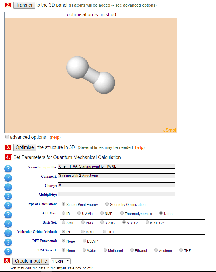
You have to go through each of the six steps on the screen.

- Build your molecule (hydrogen in step 1)
- Transfer your molecule to the 3D panel
- Optimized (this is a classical optimization)
- Set the parameters of the calculation:
- Do a single point calculation
- Use the 6-31G* basis set
- Use the Restricted Hartree-Fock (RHF) method (this will be discussed later in the course)
- Use no DFT Functional
- Use no (PCM) Solvent
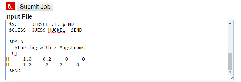
- Create the Input file (and edit it so that the atoms positions are set with a 0.2 angstrom distance in the box like below). This is one way to do it (but you can rotate your molecule any way you want in the calculations)

Then you submit
The Easy Way
Type in 02588 in the "Read Geometry From a Previous Job" and press input. It pulls in all details from a previous calculation.

Scroll down to step 4
Type a name for your file, e.g. "H2_yourname" in step 4 "Name for input file"
Check "Single-Point Energy" next to "Type of Calculation" This will instruct GAMESS not to change your coordinates.
Click "Create input file" (step 5)
Click "Submit Job" (step 6). This may take a minute or two.
The difference between single-point calculations and geometry optimization is that that the former calculates the electron structure for one specific and given geometry; the later will do it at a series of geometries while decreasing the total energy of the system.
The Output
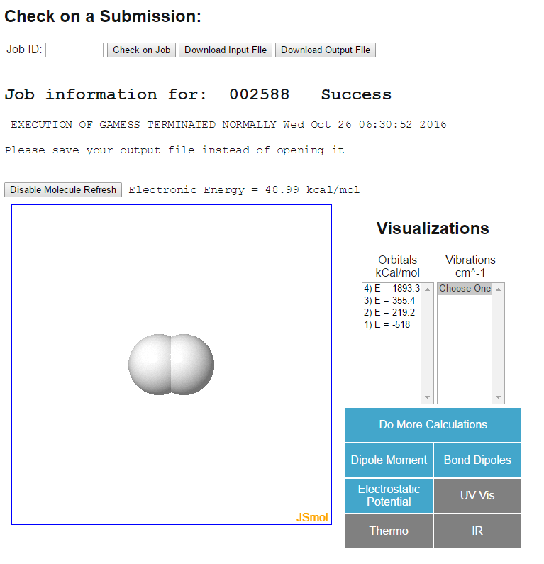
The output will look like this

There are many interesting aspects to this calculations, but for now, we are focusing on the "Electronic Energy" right above the molecule. Later on we will review the (molecular) orbitals and other cool things you can calculate. Set the energy units to kcal/mol (right above the molecule).
Build the Potential \(V(x)\) for \(H_2\) Vibration
You will construct the potential curve for molecular hydrogen one geometry point at a time (this is the Born-Oppenheimer approximation that we will learn soon). This is the "true" potential without any approximations like the harmonic oscillator or Morse oscillator potentials. It is a numerical potential and is inserted into the vibration Schrödinger equations to solve for the wavefunctions and energies via numerical approaches.
To do this you must vary the bond length. From the output of your job do this by:
- Note the electronic energy (change the units to kcal/mol)
- Click "Do More Calculations"
- Click "Manually alter coordinates"
- Double check the bond length for this calculation (calculate the distance between the two atoms)
- Vary the distance between the two atoms by editing the coordinates. It's easiest to place one atom at the origin.
- Check "Single-Point Energy" next to "Type of Calculation" This will instruct GAMESS not to change your coordinates.
- Click "Create Input File"
- Click "Submit Job"
- When the job is finished ("Success") repeat from step 1
For each bond length you will enter the electronic energy in the following table:
| Bond Length (Angstroms) | Energy (Kcal/mol) for \(H_2\) |
|---|---|
| 0.2 | 48.99 |
| 0.25 | |
| 0.3 | |
| 0.35 | |
| 0.4 | |
| 0.5 | |
| 0.6 | |
| 0.7 | |
| 0.8 | |
| 0.9 | |
| 1.0 | |
| 1.1 | |
| 1.2 | |
| 1.3 | |
| 1.4 | |
| 1.5 | |
| 2 | |
| 3 | |
| 4 | |
| 5 | |
| 6 | |
| 7 |
To be Submitted for Credit:
- Submit the above table filled out for the electronic energy of each bond length (do not copy from others as if we will compare tables)
- Plot up this potential energy curve on your favorite software (E.g., excel or matlab)
- From this plot, answer these two questions:
- What is the equilibrium bondlength for \(H_2\)?
- What is the bond energy (well depth) for \(H_2\)?
Closing Thoughts
If you are good with math and numerical analysis, you can go one step further and fit a parabolic potential (i.e., a quantum Harmonic Oscillator) to the experimental curve and extract a "spring constant" for this vibration. If you do this from these data, we will be impressed. More so if you fit a Morse oscillator to the data.

