History of Isotopes

History of the Idea of Isotopes

When we think of isotopes, we usually think of radioactive decay, which was first associated with transmutation of elements by Ernest Rutherford and Frederick Soddy in 1902^[1]. Radioactivity led to the radical modification of Dalton's Atomic Theory, because it became clear that atoms were not immutable, that they were not indivisible, and that elements consisted of more than one kind of atom.

The products of transmutations were sometimes themselves radioactive, but eventually they decay to stable atoms. Three decay series for "primordial nuclides" (those preexisting on Earth) were elucidated by Rutherford and Soddy: The series starting with \({}_{\text{92}}^{\text{238}}\text{U}\) terminated with stable "radium G" after about 20 decays; \({}_{\text{90}}^{\text{232}}\text{Th}\) decay terminated with "thorium D"; and \({}_{\text{92}}^{\text{238}}\text{U}\) decay terminated with "actinium D".

Isotopes

Soddy suggested (here, in his own words) that the final products "radium G", "thorium D", and "actinium D" were not three new elements as originally thought, but three different stable isotopes of lead \({}_{\text{82}}^{\text{206}}\text{Pb}\), \({}_{\text{82}}^{\text{207}}\text{Pb}\), \({}_{\text{82}}^{\text{208}}\text{Pb}\) with differing masses ^[2].

Figure \(\PageIndex{1}\) Frederick Soddy

 

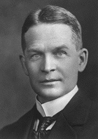
This conclusion was reached simultaneously in 1913 by Kasimir Fajans (1887-1975) and Soddy (1877-1956). Fajans called the chemically identical atoms with differing isotopic masses pleiads, but Soddy called them Isotopes, the name we currently use. Here it is in Soddy's words, where he argues against Fayan's idea that isotopes are distinguished by electronic changes (eg. ₉₀U⁴⁺ would be identical to ₉₀Th²⁺). At the time, neutrons were unknown, and atoms were thought to be pairs of positive and negatively charged particles.The Nobel Prize in Chemistry 1921 was awarded to Frederick Soddy "for his contributions to our knowledge of the chemistry of radioactive substances, and his investigations into the origin and nature of isotopes"^[3].

\

Table \(\PageIndex{1}\) Four stable isotopes of lead.

Isotope	Symbol	Protons	Neutrons	% on Earth	Isotopic Mass
lead-204	\({}_{\text{82}}^{\text{204}}\text{Pb}\)	82	122	1.40%	203.973
lead-206	\({}_{\text{82}}^{\text{206}}\text{Pb}\)	82	124	24.10%	205.974
lead-207	\({}_{\text{82}}^{\text{207}}\text{Pb}\)	82	125	22.10%	206.976
lead-208	\({}_{\text{82}}^{\text{208}}\text{Pb}\)	82	126	52.40%	207.977

Isotopic Abundances

Atomic weights were determined by the chemical combining ratio method, refined and optimized by Theodore William Richards (1868-1928). The method was still time consuming, and Soddy's identification of isotopes was laborious. Lead from different sources did indeed have different atomic weights, from Richards publication in 1914. Common lead was 207.15; lead from North Carolina uraninite was 206.40, but a thorite from Honigschmid gave the highest value, 207.90.

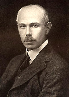
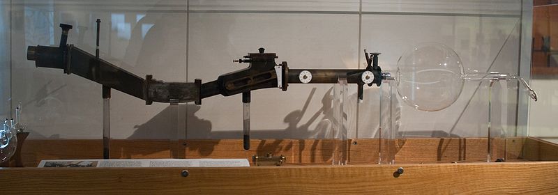
J.J. Thompson noticed that canal rays for a single element were deflected by a magnetic field to give two traces on a fluorescent screen, and his assistant, Francis William Aston (1877-1945) further developed the technique, building the first mass spectrograph in 1919. This instrument gave both the mass (from particle deflection) and abundance (from exposure of a photographic plate) of ions very precisely. Aston won the [Nobel Prize:http://nobelprize.org/nobel_prizes/chemistry/laureates/1922/aston-bio.html 1922 Nobel Prize in Chemistry] for his development of mass spectometry, as described in his own words here.

Figure \(\PageIndex{2}\) Francis William Aston

But is there a "normal" isotopic abundance ratio for an element? If the abundance of oxygen isotopes can vary by ~20‰ (2%), how can we have a single "atomic weight" for the element?

The "Normal" Isotopic Ratio: Atomic Weights

All atoms of a given element do not necessarily have identical masses. But all elements combine in definite mass ratios, so they behave as if they had just one kind of atom. In order to solve this dilemma, we define the atomic weight as the weighted average mass of all naturally occurring (occasionally radioactive) isotopes of the element.

A weighted average is defined as

Atomic Weight =

\(\left(\dfrac{\%\text{ abundance isotope 1}}{100}\right)\times \left(\text{mass of isotope 1}\right)~ ~ ~ +\)

\(\left(\dfrac{\%\text{ abundance isotope 2}}{100}\right)\times \left(\text{mass of isotope 2}\right)~ ~ ~ + ~ ~ ...\)

Similar terms would be added for all the isotopes. Since the abundances change from place to place, IUPAC has established "normal" abundances which are most likely to be encountered in the laboratory. This important document that reports these values can be found at the IUPAC site. The abundances are also usually listed on the Table of the Nuclides which lists all isotopes for all elements. Surprisingly, a good number of elements have isotopic abundances that vary quite widely, so that atomic weights based on them have only 3 or 4 digit precision.

The atomic weight calculation is analogous to the method used to calculate grade point averages in most colleges:

GPA =

\(\left(\dfrac{\text{Credit Hours Course 1}}{\text{total credit hours}}\right)\times \left(\text{Grade in Course 1}\right)~ ~ ~ +\)

\(\left(\dfrac{\text{Credit Hours Course 2}}{\text{total credit hours}}\right)\times \left(\text{Grade in Course 2}\right)~ ~ ~ + ~ ~ ...\)

Example \(\PageIndex{1}\): The Atomic Weight of Lead

Calculate the atomic weight of an average naturally occurring sample of lead from the data in the table above.

Atomic Weight = \(\dfrac{\text{1.40%}}{\text{100}} \times \text{203.973} + \dfrac{\text{24.10%}}{\text{100}} \times \text{205.947} + \dfrac{\text{22.10%}}{\text{100}} \times \text{206.976} + \dfrac{\text{52.40%}}{\text{100}} \times \text{207.997} =\text{207.22}\)

Example \(\PageIndex{2}\): Isotopic Mass of Carbon

Naturally occurring carbon is found to consist of two isotopes:

Isotope	Symbol	Protons	Neutrons	% on Earth	Isotopic Mass
Carbon-12	\({}_{\text{6}}^{\text{12}}\text{C}\) 12	6	6	98.93%	12.0000000
Carbon-13	\({}_{\text{6}}^{\text{13}}\text{C}\)	6	7	1.07%	13.0033548

Solution

\[\dfrac{\text{98.93}}{\text{100.00}} \times \text{12.00} + \dfrac{\text{1.07}}{\text{100.00}} \times \text{13.0034} = \text{12.011}\nonumber\]

The exact isotopic mass of \({}_{\text{6}}^{\text{12}}\text{C}\) may be surprising. It is assigned the value 12.0000000 as a standard for the atomic weight scale. Other masses are determined by mass spectrometers calibrated with this arbitrary standard.

Defining the Mole

The SI definition of the mole also depends on the isotope \({}_{\text{6}}^{\text{12}}\text{C}\) and can now be stated. One mole is defined as the amount of substance of a system which contains as many elementary entities as there are atoms in exactly 0.012 kg of 126C. The elementary entities may be atoms, molecules, ions, electrons, or other microscopic particles. This official definition of the mole makes possible a more accurate determination of the Avogadro constant than was reported earlier. The currently accepted value is N_A = 6.02214179 × 10²³ mol^–1. This is accurate to 0.00000001 percent and contains five more significant figures than 6.022 × 10²³ mol^–1, the number used to define the mole previously. It is very seldom, however, that more than four significant digits are needed in the Avogadro constant. The value 6.022× 10²³ mol^–1 will certainly suffice for most calculations needed.

history en.Wikipedia.org/wiki/Frederick_Soddy Frederick Soddy names isotopes; p. 137 Hudson; p. 172: Francis William Aston's mass spec Theodore William Richards Atomic Weight Determinations

From ChemPRIME: 4.13: Average Atomic Weights

References

1. ↑ http://web.lemoyne.edu/~giunta/ruthsod.html
2. ↑ Hudson, J. "The history of Chemistry", Chapman & Hall, NY, 1992, p. 170
3. ↑ http://nobelprize.org/nobel_prizes/chemistry/laureates/1921/soddy-bio.html#

Contributors and Attributions

• Ed Vitz (Kutztown University), John W. Moore (UW-Madison), Justin Shorb (Hope College), Xavier Prat-Resina (University of Minnesota Rochester), Tim Wendorff, and Adam Hahn.