3.7: The Golden Rule

\( \let\bibref\eqref   %make-command_bibref-equivalent-to-eqref\)\(\newcommand \sinc{\text{sinc}}\)Several important relationships in quantum mechanics that describe rate processes come from time-dependent perturbation theory. The Golden Rule, typically attributed to Fermi even though Dirac first developed it, refers to a series of expressions from first-order perturbation theory that describe the population transfer rate from one quantum state to another that arise from applying an external potential that couples the two states. Specifically, these expressions apply if the changes in the population of the states is very small, and we only consider direct coupling between the initial and final state. As we will see, there are many ways in which these expressions can be written and applied. The important results are derived from two model problems that we want to work through: (1) time evolution after applying a step perturbation, and (2) time evolution after applying a harmonic or sinusoidal perturbation.

As before, the Hamiltonian for the problem takes the form \(H=H_0+V(t)\), where \(H_0\) is the time-independent Hamiltonian for the system we are observing, and \(V(t)\) is an external potential which we apply to the system. Again, we will ask: if we prepare the system in the state \(\left| \ell \right\rangle\), an eigenstate of \(H_0\), what is the probability of observing the system in state \(\left| k \right\rangle\) following the perturbation? In both cases, we will abruptly turn on a perturbation at time \(t_0=0\).

Constant perturbation

Figure \(\PageIndex{1}\)

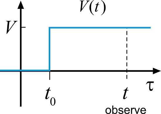
For the first model calculation, we simply apply a step perturbation, during on a constant potential of amplitude \(V\) at time \(t_0\):

\[V\left( t \right) = \left\{ \begin{array}{*{20}{c}} 0\quad t < t_{0}\\ V\quad t \ge t_{0} \end{array} \right.\label{eq3.7.1}\]

and evaluate the resulting state amplitude in other states \(k\), with the first order expression, eq. (\(3.6.6\)):

\[b_{k} = - \frac{i}{\hbar }\int_{t_{0}}^{t} d\tau \;e^{i\omega _{k\ell }(\tau - t_{0})}\,V_{k\ell }\label{eq3.7.2}\]

The matrix element \(V_{k\ell } = \left\langle k \right|V\left| \ell \right\rangle\) is independent of time, and the only time-dependence arises from switching on the perturbation. Setting \(t_0=0\), we can evaluate this expression as

\[\begin{array}{rl} b_{k}  \kern-.8em & \displaystyle = - \frac{i}{\hbar }V_{k\ell }\int_{0}^{t} d\tau \; e^{i\omega _{k\ell }\tau }\\ & \displaystyle = - \frac{V_{k\ell }}{E_{k} - E_{\ell }}\left[ \exp \left( i\omega _{k\ell }t \right) - 1 \right] \end{array}\label{eq3.7.3}\]

We now make use of an identity that is helpful to evaluate population changes:

\[e^{i\theta } - 1\; = \;2i\,e^{i{ \theta / 2 }}\sin \left( \frac{\theta }{2} \right)\label{eq3.7.4}\]

With this expression, the time-dependent amplitude of state \(k\) is

\[b_{k} = - \frac{2i\,V_{k\ell }\;e^{i\omega _{k\ell }t/2}}{E_{k}\,\; - \;E_{\ell }}\;\sin \left( \frac{1}{2}\omega _{k\ell }t \right)\label{eq3.7.5}\]

and the corresponding population in state \(k\) is obtained from

\[P_{k} = \left| b_{k} \right|^{2} = \frac{4\left| V_{k\ell } \right|^{2}}{\left| E_{k} - E_{\ell } \right|^{2}}\;\sin ^{2}\left( \frac{1}{2}\omega _{k\ell }t \right)\label{eq3.7.6}\]

We observe that the abrupt application of a constant perturbation induces a sinusoidal transfer of population between states \(k\) and \(\ell\) with an amplitude that depends on the magnitude of the purturbation matrix element squared. If we write this using the energy splitting variable we used earlier,

\[\Delta = \frac{E_{k} - E_{\ell }}{2}\label{eq3.7.7}\]

then

\[P_{k}\; = \;\frac{V^{2}}{\Delta ^{2}}\;\sin ^{2}\left( \frac{\Delta \,}{\hbar }t \right)\label{eq3.7.8}\]

We can compare this with the exact result for the two-level problem that we solved in Section ZZZ:

\[P_{k}\; = \;\frac{V^{2}}{V^{\mathbf{2}} + \Delta ^{2}}\;\sin ^{2}\left( \frac{\sqrt {\Delta ^{2} + V^{2}\,} \,}{\hbar }t \right)\label{eq3.7.9}\]

As expected, the perturbation theory result works well when the magnitude of the perturbation is small compared to the energy gap, \(V\ll\Delta\), which also corresponds to cases where the population change in the system is small, \(P_k\ll1\).

Looking more carefully, in Figure \(3.7.2\) we examine the time-dependence to \(P_k\) and compare the perturbation theory (solid lines) to the exact result (dashed lines) for different values of \(\Delta\). The correspondence is poor at \(\Delta=0\), for which \(P_k\) grows quadratically and the probability quickly exceeds unity. It’s certainly unrealistic, but not surprising, since we don’t expect that the expression will hold for the “strong coupling” case: \(\Delta\ll\ V\). One begins to have quantitative accuracy in for the regime \(P_k\left(t\right)-P_k(0)<0.1\) or \(\Delta<4V\). Next, let’s plot this a little differently in Figure 9b, scaling the time axis as \(2\pi\hbar/\Delta\), focusing on the changes for \(t\ll\Delta/\hbar\), and looking at \(\sqrt{P_k}\), the magnitude of the expansion coefficient \(\left|b_k\right|\). Here we see that the first-order perturbation theory result is excellent at describing the initial changes as amplitude flows into the target state \(|k\rangle\), particularly for small changes \({|b}_k\left(t\right)|^2<0.1\).

Figure \(\PageIndex{2}\): (a) Comparison of the time-dependent population of target state \(\left| k\right\rangle\) as a function of time from the exact two-level system result, eq. (\ref{eq3.7.9}), in dashed lines with that from first-order perturbation theory, eq. (\ref{eq3.7.8}), in solid lines. (b) Changes in the amplitude in \(b_k\) the coefficient for the target state for short times illustrating linear growth and good correspondence of first-order perturbation theory with exact result.

Now let’s look at how the population transfer to state \(k\) depends on both \({\rm{\Delta }}\) and \(t\). Using \(\sinc \kern-.1em \left( x \right) = \sin \left( x \right)/x\), we can rewrite the first-order result in eq. (\ref{eq3.7.8}) as

\[P_{k}\; = \frac{V^{2}t^{2}}{\hbar ^{2}}\sinc ^{2}\left( \frac{\Delta \,}{\hbar }t \right)\label{eq3.7.10}\]

A plot of the corresponding population transferred from \(\left| \ell \right\rangle\) to \(\left| k \right\rangle\) is shown in Figure 10 as a function of the detuning \({\rm{\Delta }}\). The probability of transfer peaks sharply where the energy of the initial state matches that of the final state, and, over time, efficient transfer requires a narrower energy difference between initial and final states. To examine the time-dependent behavior of \(P_k\), we use \(\mathop \lim \limits_{x \to 0} \;\sinc \left( x \right) = 1\), to show that the probability grows quadratically at short time spans:

\[\mathop \lim \limits_{\Delta \to 0} P_{k} = { V^{2}t^{2} / \hbar ^{2} }\label{eq3.7.11}\]

Since \(P_k\) will exceed 1, this is clearly non-physical behavior. This serves to illustrate that first-order perturbation theory only applies to small changes in amplitude and for times spans in which feedback of the amplitude back into the initial state is not yet significant.

Figure \(\PageIndex{3}\): Illustration of the efficiency of the efficiency of population transfer to the target state \(|k\rangle\) as a function of time following the onset of the constant perturbation. The first-order perturbation theory result (solid line) is compared with the exact result (dashed line).

From eq. (\ref{eq3.7.10}) we may observe that the spread of final state energies to which transfer remains possible narrows with time at a rate of \(t^{-1}\): \(E_{k} - E_{\ell } < { 2\pi \hbar / t }\). If the perturbation continues long enough, the energies of the two states must be equal. This observation is sometimes referred to as a time-energy uncertainty relation, where \(\Delta E \cdot \Delta t \ge 2\pi \hbar\). However, remember that this is just an observation of the principles of Fourier transforms. A frequency, and thereby energy, can only be determined as accurately as the length of the time over which we observe oscillations. Since time is not an operator, time and energy do not have a quantum uncertainty relation like \(\Delta p \cdot \Delta x \ge 2\pi \hbar\), which derives from the fact that \(p\) and \(x\) do not commute.

In the long-time limit, the \(\sinc^2 (x)\) function narrows to a delta function according to

\[\mathop \lim \limits_{a \to \infty } \frac{\sin ^{2}\left( { ax / 2 } \right)}{ax^{2}} = \frac{\pi }{2}\;\delta \left( x \right)\label{eq3.7.12}\]

and the population in state \(k\) is observed to grow linearly with time:

\[\mathop \lim \limits_{t \to \infty } P_{k}\left( t \right) = \frac{2\pi }{\hbar }\;\left| V_{k\ell } \right|^{2}\delta \left( E_{k} - E_{\ell } \right)\;t\label{eq3.7.13}\]

The delta function enforces energy conservation, saying that the energies of the initial and target state must be the same in the long-time limit. Of course, this expression is also unphysical since \(P_k\) can exceed 1 on long enough time scales.

What is interesting in eq. (\ref{eq3.7.13}) is that a linear growth of population with time indicated that the transfer rate \(w_{k} = { \partial P_{k} / \partial t }\) is independent of time, as expected for a rate constant in simple first-order kinetics. This population transfer rate is

\[w_{k} = \frac{2\pi }{\hbar }\;\left| V_{k\ell } \right|^{2}\delta \left( E_{k} - E_{\ell } \right)\label{eq3.7.14}\]

That is, the rate at which population leaves \(\ell\) and grows into state \(k\) is simply related to the square of the matrix element for the perturbation, in addition to requiring that the initial and final states have the same energy. This is one statement of the Golden Rule—the state-to-state form for a constant perturbation—which describes energy transfer and relaxation rates from first-order perturbation theory. In fact we will find that more accurate and complex treatments of the state-to-state transfer rate that properly conserve the probability amplitude of the system still predict the same rate constant as eq. (\ref{eq3.7.14}). We will show that this rate properly describes the long time exponential decay observed for irreversible relaxation processes that we would expect from the solution of the rate equation \({ dP / dt } = - w{\kern 1pt} P\).

It is worth noting that the result that we obtained in eq. (\ref{eq3.7.14}) is independent of the manner in which the perturbation is switched on. It may seem unphysical to turn on a perturbation instantaneously or that it matters whether the switch happens slowly; however, once we evaluate the \(t\rightarrow\infty\) limit, the resulting rate expression is independent of the way the perturbation is applied.

Like time-independent perturbation theory, it is possible that the matrix element for first-order transitions \(V_{k\ell}\) is zero, and that second-order perturbation theory is needed to describe the primary interactions that couple the initial and final states. This would apply to cases in which an intermediate state \(|m\rangle\) mediates the transfer of probability amplitude from \(|\ell\rangle\) to \(\left|k\right\rangle\). Under those circumstances, one can derive a similar Golden Rule expression for the rate of transfer from \(\ell\) to \(k\) through \(m\) using the strategies described above, and one obtains \(\bibref{Cite1} %in-text-citation\)

\[w_{\ell \to m \to k} = \frac{2\pi }{\hbar }\left| \frac{V_{km}V_{m\ell }}{E_{\ell } - E_{m}} \right|^{2}\delta \left( E_{k} - E_{\ell } \right)\label{eq3.7.15}\]

If there are multiple intermediate states—either discrete or a continuum—one can sum this expression over the continuum of states that contribute to the transfer using \(\Sigma_mw_{\ell\rightarrow\ m\rightarrow\ k}.\)

Population transfer to a continuum

Since first-order perturbation theory does not allow population feedback between the initial and final states, it turns out to be most useful in cases where we are interested in the rate of leaving an initial state. The Golden Rule is particularly useful for irreversible processes in which an initially prepared state transfers population amplitude continuum of accepting states, which we describe in Sec. YYYY. Examples include (1) the ionization of atoms in an electric field where the continuum are free particle waves, spontaneous emission of light by electronically excited molecules where the continuum of states are electromagnetic waves of varying frequency, and vibrational energy dissipation to a bath of phonons. Although dynamics of interactions with continua won’t come up much until we tackle condensed matter problems, this is a good point to discuss how the Golden Rule rates are expressed for the case of state-to-continuum rate processes.

As in the prior section, we will calculate the transition probability from initial state \(\left| \ell \right\rangle\) to a continuum of final states, \(\left\{|k\rangle\right\}\). If \(P_\ell\) is the probability of occupying the initial state, then the probability of occupying any state in the continuum is \({\bar{P}}_k=1-P_\ell\). \({\bar{P}}_k\) then can be expressed as the sum of probabilities for occupying a particular state within the continuum: \(\bar{P}=\Sigma_kP_k\). The rates of transfer from \(\ell\) to a specific state \(k^\prime\) is again obtained from \(w_{k^\prime\ell}=\partial\ P_{k\prime}/\partial\ t\). Since first order perturbation theory only concerns itself with the rate of leaving state \(\ell\), the rate of transfer to all continuum states is merely a sum of the rates to each state:

\[\bar w_{k\ell } = \;\sum\limits_{k} w_{k\ell } \label{eq3.7.16}\]

For a continuum, the sum over discrete states can be replaced by an integral over a density of states \(\rho \left( E_{k} \right)\) that describes the number of continuum states per energy interval:

\[\bar w_{k\ell } = \int dE_{k}\;\rho \left( E_{k} \right)\;w_{k\ell }\left( E_{k} \right) \label{eq3.7.17}\]

where \(w_{k\ell}\) is given by eq. (\ref{eq3.7.13}). One can evaluate this integral if one can make two simplifying assumptions: (1) \(\rho \left( E_{k} \right)\) varies slowly enough to be a constant and can be removed from the integral. (2) The matrix element \(V_{k\ell }\) connecting initial and final states is the same for all states within the continuum. These assumptions are typically reasonable when one is working within the weak coupling requirement of perturbation theory. Then eq. (\ref{eq3.7.17}) becomes

\[\bar w_{k\ell }\; = \;\frac{2\pi }{\hbar }\;\;\left| V_{k\ell } \right|^{2}\rho \left( E_{\ell } \right)\label{eq3.7.18}\]

Thus the rate of transfer of population to the continuum depends only on the matrix element squared for the interaction of state \(\ell\) and continuum states, and the density of accepting continuum states at the energy of the initial state. This is the common state-to-continuum form of the Golden Rule used often in the calculation of chemical and relaxation rate processes.

Harmonic perturbation

The second model calculation is to determine the transfer of population from state \(\ell\) to \(k\) after turning on a harmonic or sinusoidal perturbation at time \(t_{0}\). The results are important for spectroscopy, since they will be used to describe how electromagnetic fields induce transitions between quantum states of the system. In this case, we turn on an external potential that oscillates with an angular frequency \(\omega\) and the magnitude of the perturbation is governed by \(V_{0}\).

\[V(t) = V_{0}\cos \omega t \qquad (t\geq\ t_0)\label{eq3.7.19}\]

Figure \(\PageIndex{4}\): Illustration of the sudden onset of a sinusoidal perturbation of magnitude \(V\) at time \(t_0\).

\(V_{0}\;\) can be expressed in terms of operators of the system, so the matrix elements of the interaction potential are given by

\[V_{k\ell }\left( t \right) = V_{k\ell }\cos \omega t\label{eq3.7.20}\]

where \(V_{k\ell } = \langle k\left| V_{0} \right|\ell \rangle\). Note that our results are independent of the phase of this wave, so using a \(\sin \omega t\) form will return the same key results.

To calculate resulting probability amplitude in state \(k\) we again make use of our first order expression, eq. (\(3.6.6\)), and express the cosine in its complex form: \(\cos \omega t = {\textstyle{1 \over 2}}\left[ e^{ - i\omega t} + e^{i\omega t} \right]\). Setting \(t_{0} \to 0\), we obtain:

\[\begin{array}{rl} b_{k}  \kern-.75em & \displaystyle = \frac{ - i}{\hbar }\int_{t_{0}}^{t} d\tau \;V_{k\ell }\left( \tau \right)\;e^{i\omega _{k\ell }\tau }\\
&= \displaystyle  \frac{ - iV_{k\ell }}{2\hbar }\int_{0}^{t} d\tau \;\left[ e^{i\left( \omega _{k\ell } - \omega \right)\tau }\; + e^{i\left( \omega _{k\ell } + \omega \right)\tau } \right]\\
& \displaystyle = - \frac{V_{k\ell }}{2\hbar }\;\left[ \frac{e^{i\left( \omega _{k\ell } - \omega \right)t}\, - \,1}{\omega _{k\ell } - \omega }\; + \frac{e^{i\left( \omega _{k\ell } + \omega \right)t}\, - \,1}{\omega _{k\ell } + \omega }\; \right] \end{array}\label{eq3.7.21}\]

Then using identity (\ref{eq3.7.4}), we get

\[b_{k} = \frac{iV_{k\ell }}{\hbar }\left[ \frac{e^{i{ \left( \omega _{k\ell } - \omega \right)t / 2 }}\;\sin \left[ {\textstyle{1 \over 2}}\left( \omega _{k\ell } - \omega \right)t \right]}{\omega _{k\ell } - \omega } + \;\frac{e^{i{ \left( \omega _{k\ell } + \omega \right)t / 2 }}\;\sin \left[ {\textstyle{1 \over 2}}\left( \omega _{k\ell } + \omega \right)t \right]}{\omega _{k\ell } + \omega } \right]\;\label{eq3.7.22}\]

This expression has many omegas, so it is worth reiterating that \(\omega\) is the frequency of the harmonic perturbation and is positive, whereas \(\omega _{k\ell } = \left( E_{k} - E_{\ell } \right)/\hbar\) reflects the energy splitting between the initial and final states and can be positive or negative. It is also worth noting that when we set \(\omega \to 0\) that we do recover the expected behavior from the constant perturbation in eq. (\ref{eq3.7.5}). This observation suggests a mathematical advantage for solving certain time-dependent problems with Fourier transformations over a sinusoidal potential and then applying the \(\omega \to 0\) limit at the end.

Figure \(\PageIndex{5}\): Energy level diagram illustrating the changes in the system corresponding to the two terms in eq. (\ref{eq3.7.22}).

The denominators in eq. (\ref{eq3.7.22}) indicate that the two terms only have a significant impact on the system when \(\omega \; \approx \;\left| \omega _{k\ell } \right|\). This condition for efficient transfer is resonance, a matching of the frequency of the harmonic interaction with the energy splitting between quantum states. Consider the resonance conditions that will maximize each of these two terms. The first term in eq. (\ref{eq3.7.22}) is maximized when \(\omega = \omega _{k\ell }\), which occurs when \(E_{k} > E_{\ell }\), and thus transfer of population from \(\ell\) to \(k\). requires an input of energy from the external potential by an amount \(\hbar \omega\). This term is therefore referred to as absorption. The second term is maximized when \(\omega = - \omega _{k\ell }\), which occurs when \(E_{k} < E_{\ell }\), corresponding to a loss of energy by the system by an amount \(\hbar \omega\). This term is often called stimulated emission due to its role in spectroscopy. In a quantum description of spectroscopy, we associate the increase of energy in the system on absorption with a loss of a quantum of energy \(\hbar \omega\) in the light field, a photon. Similarly, the loss of energy in the system is related to the creation of a photon with energy \(\hbar \omega\) in the light field. Thus, when considering both the light and matter, the total energy is conserved. However, our current first order perturbation theory description of the matter does not concern itself with the state of the light field; the potential is assumed to be unchanged by what happens in the system, so the energy of the system need not be conserved.

If we consider absorption only, we can use the first term in eq. (\ref{eq3.7.22}) to calculate the time-dependent probability of occupying state \(k\)

\[P_{k}\; = \;\left| b_{k} \right|^{2}\; = \;\frac{\left| V_{k\ell } \right|^{2}}{\hbar ^{2}\left( \omega _{k\ell } - \omega \right)^{2}}\quad \sin ^{2}\left[ {\textstyle{1 \over 2}}\left( \omega _{k\ell } - \omega \right)t \right]\label{eq3.7.23}\]

This expression is similar to eq. (\ref{eq3.7.6}), in that is shows that the onset of the perturbation creates an oscillatory transfer of population between the \(\ell\) and \(k\) states with an amplitude that scales as \(\left| V_{k\ell } \right|^{2}\), but it also has similar problems. In this case, the important control variable to analyze is the detuning from resonance

\[\Delta \omega = \omega _{k\ell } - \omega \label{eq3.7.24}\]

which quantifies how closely matched the frequency of the harmonic perturbation is to the energy splitting between \(\ell\) and \(k\). Rewriting eq. (\ref{eq3.7.23}) in terms of \({\rm{\Delta }}\omega\) gives:

\[P_{k}\; = \frac{\left| V_{k\ell } \right|^{2}}{\hbar ^{2}\Delta \omega ^{2}}\sin ^{2}\left[ {\textstyle{1 \over 2}}\Delta \omega \,t \right]\label{eq3.7.25}\]

To assess the validity of the perturbation theory expression, it is helpful for us to compare eq. (\ref{eq3.7.25}) with the exact expression that we derived for the driven two-level system, eq. (\(3.4.19\)):

\[P_{k}\; = \;\frac{\left| V_{k\ell } \right|^{2}}{\hbar ^{2}\Delta \omega ^{2} + \left| V_{k\ell } \right|^{2}}\sin ^{2}\left[ \frac{1}{2}\sqrt {\frac{\left| V_{k\ell } \right|^{2}}{\hbar ^{2}} + \Delta \omega ^{2}} \;t \right]\label{eq3.7.26}\]

Since perturbation theory requires small changes in population, \(P_{k} \ll 1\), eq. (\ref{eq3.7.25}) is valid for perturbations that are small relative to the detuning \(\left| V_{k\ell } \right| \ll \left| \hbar \Delta \omega \right|\). However, the exact solution also shows that we should expect the most efficient population transfer when \({\rm{\Delta }}\omega = 0\). As with the constant perturbation, eq. (\ref{eq3.7.25}) can be we-written in \(\sinc\) function form as

\[P_{k} = \frac{V_{k\ell} ^{2}\,t^{2}}{4\hbar ^{2}}{\rm{sinc}}\left( \frac{1}{2}{\rm{\Delta }}\omega \,t \right)\label{eq3.7.27}\]

In Figure \(3.7.6\), we plot the population in state \(k\) as a function of\(\)\({\rm{\Delta }}\omega\), showing that \(P_{k}\) is peaked at \({\rm{\Delta }}\omega = 0\) and the amplitude grows as \(t^{2}\). This clearly will not describe long-time behavior since it suggests unlimited growth, but it will hold for small \(P_{k}\) such that

\[t\; \ll \;\frac{2\hbar }{V_{k\ell }}\label{eq3.7.28}\]

At the same time, we cannot observe the system on too short of a time scale. We need the field to make several oscillations for this to be considered a harmonic perturbation.

\[t > \frac{1}{\omega } \approx \frac{1}{\omega _{k\ell }}\label{eq3.7.29}\]

Combining relationships (\ref{eq3.7.28}) and (\ref{eq3.7.29}) imply that perturbation theory is valid when the magnitude of the external potential’s influence is much smaller than the energy splitting between states, or \(V_{k\ell } \ll \hbar \omega _{k\ell }\).

Figure \(\PageIndex{6}\): Time-dependent population of state \(\left| k \right\rangle\) after applying the harmonic perturbation as a function of detuning from resonance.

Like our description of the constant perturbation, the long-time limit for \(P_{k}\) results in a delta function centered at \({\rm{\Delta }}\omega = 0\) and a linear increase with time.

\[\mathop \lim \limits_{t \to \infty } P_{k}\; = \frac{\pi }{2\hbar ^{2}}\left| V_{k\ell } \right|^{2}t\,\delta \left( \omega _{k\ell } - \omega \right)\label{eq3.7.30}\]

The Golden Rule rate for the rate of absorption from \(\ell\) to \(k\) is then calculated by taking the time-derivative: \(w_{k\ell } = \partial P_{k}/\partial t\):

\[w_{k\ell }\; = \;\frac{\pi }{2\hbar ^{2}}\left| V_{k\ell } \right|^{2}\,\delta \left( \omega _{k\ell } - \omega \right) \label{eq3.7-nonum1}\nonumber\]

In this limit, the one can neglect any possible interferences effects between the absorption and stimulated emission terms in eq. (\ref{eq3.7.22}). A parallel derivation of rates of stimulated emission from a higher energy state \(\ell\) to a lower energy state \(k\) results in the same expression as eq. (\ref{eq3.7.30}), except with the delta function \(\delta \left( \omega _{k\ell } + \omega \right)\). As a result, the total rate of transitions induced by a harmonic perturbation from an initial state \(\ell\) to a final state \(k\) independent of which state is higher in energy is

\[w_{k\ell }\; = \;\frac{\pi }{2\hbar ^{2}}\,\left| V_{k\ell } \right|^{2}\;\left[ \delta \left( \omega _{k\ell } - \omega \right)\; + \;\delta \left( \omega _{k\ell } + \omega \right) \right]\label{eq3.7.31}\]

This is the state-to-state form of the Golden Rule for a harmonic perturbation, an important result we will use in our description of light-matter interactions and spectroscopy. In practice, state-to-state expressions typically need to be summed over the set of all possible final states \(\{\left| k\right\rangle\}\) accessible to direct transitions from \(\left| \ell \right\rangle\). For ensembles, one also needs to sum over the distribution of initial states weighted by their initial population.

Time-domain derivation

Different routes can be taken to obtain the Golden rule, but often it is hard to retain the physical picture that links the characteristics of the time-dependent potential and the rates of population transfer. An alternate approach can be used to obtain a time-domain representation of the state-to-state expressions for the Golden Rule. In this case, we calculate the rate as the time-dependent change of the population in state \(\left| k \right\rangle\) working directly from

\[w_{k\ell } = \frac{dP_{k\ell }}{dt}\label{eq3.7-nonum2}\nonumber\]

Since the population of state \(k\) is \(P_{k\ell } = \left| b_{k} \right|^{2} = b_k^{*}b_{k}\), we can expand this equation in the time-derivatives of \(b_{k}\) as

\[w_{k\ell } = \frac{d}{dt}\left( b_k^{*}b_{k} \right) = \dot b_k^{*}b_{k} + b_k^{*}\dot b_{k}\label{eq3.7.32}\]

The first-order expressions for \(b_{k}(t)\) and \(\dot b_{k}(t)\) are given by eqs. (\(3.6.6\)) and (\(3.6.7\)), respectively. Using the fact that our initial state is \(\ell\) and \(b_{\ell }(0) = 1\), we can write the first term in eq. (\ref{eq3.7.32}) as

\[\begin{array}{c} \dot b_k^{*}b_{k} = \displaystyle \frac{i}{\hbar }V_{k\ell} ^{\dagger}(t)e^{ - i\omega _{k\ell }t}\frac{ - i}{\hbar }\int_{0}^{t} dt'\,V_{k\ell }(t')e^{i\omega _{k\ell }t'} \\
 = \displaystyle \frac{1}{\hbar ^{2}}\int_{0}^{t} dt'\,V_{k\ell} ^{\dagger}(t)V_{k\ell }(t')e^{i\omega _{k\ell }(t' - t)} \end{array}\label{eq3.7.33}\]

Since we are investigating the long-time behavior upon application of the perturbation relevant to the Golden Rule, we can set the upper integration limit to \(t \to \infty\). Next we substitute the time-interval variable \(\tau = t' - t\) and make use of the stationary property of time-propagators

\[\begin{array}{rl} \dot b_k^{*}b_{k}  \kern-.75em  & \displaystyle = \frac{1}{\hbar ^{2}}\int_{0}^{t} d\tau \,V_{k\ell} ^{\dagger}(t)V_{k\ell }(\tau + t)e^{i\omega _{k\ell }\tau } \\
& \displaystyle = \frac{1}{\hbar ^{2}}\int_{0}^{t} d\tau \,V_{k\ell} ^{\dagger}(0)V_{k\ell }(\tau )e^{i\omega _{k\ell }\tau } \end{array}\label{eq3.7.34}\]

Repeating this for the second term in eq. (\ref{eq3.7.32}) gives

\[b_k^{*}\dot b_{k} = \frac{1}{\hbar ^{2}}\int_{0}^{t} d\tau V_{k\ell} ^{\dagger}(\tau )V_{k\ell }(0)e^{ - i\omega _{k\ell }\tau } \label{eq3.7.35}\]

We can observe that the differences between these two similar terms are the arguments of their exponentials and the sequence of the operators over which we integrate. One term is the complex conjugate of the other, as one would expect from \(P_{k\ell }\) being real. One can obtain the result directly from taking the real part of either expression, but it is more useful to combine the two integrals. Taking the long-time limit (\(t \to \infty\)) of the combined integral, we find that the transition rate is

\[w_{k\ell } = \frac{1}{\hbar ^{2}}\int_{ - \infty }^{\infty } d\tau \,V_{k\ell }(\tau )V_{\ell k}(0)e^{i\omega _{k\ell }\tau } \label{eq3.7.36}\]

This is a time-domain representation of Fermi’s Golden rule which takes the form of a Fourier transform over a correlation function for the time-dependent variation of the coupling matrix elements \(V_{k\ell }\left( t \right)\). It equates the efficiency of making transitions between two states to the Fourier component at the energy gap between coupled states, \(\omega _{k\ell }\;\). This is an important result that will return to often.

To connect this expression to our prior results, consider the case of a constant perturbation in which the matrix elements are time independent, and we obtain

\[w_{k\ell } = \frac{1}{\hbar ^{2}}\left| V_{k\ell } \right|^{2}\int_{ - \infty }^{\infty } d\tau \,e^{ - i\omega _{k\ell }\tau } \label{eq3.7.37}\]

The integral in this equation is \(2\pi \delta \left( \omega _{k\ell } \right)\). This allows eq. (\ref{eq3.7.37}) to be written as eq. (\ref{eq3.7.14}). If we instead take the interaction potential to have a harmonic time-dependence, the same procedure results in eq. (\ref{eq3.7.31}). The time-domain expression, eq. (\ref{eq3.7.36}), will play an increasingly important role in describing how molecular dynamics influence rate processes and spectroscopy as we move forward.

---

References

\(\tag {1} \label {Cite1}\)

Baym, G., Lectures on Quantum Mechanics. Perseus Book Publishing, L.L.C.: New York, 1969; p. 257.

Readings

\(\tag {2} \label {Cite2}\)	Cohen-Tannoudji, C.; Diu, B.; Lalöe, F., Quantum Mechanics. Wiley-Interscience: Paris, 1977; p. 1299.
\(\tag {3} \label {Cite3}\)	McHale, J. L., Molecular Spectroscopy. 1st ed.; Prentice Hall: Upper Saddle River, NJ, 1999; Ch. 4.
\(\tag {4} \label {Cite4}\)	Sakurai, J. J., Modern Quantum Mechanics, Revised Edition. Addison-Wesley: Reading, MA, 1994.